www.atmos-meas-tech.net/4/409/2011/ doi:10.5194/amt-4-409-2011
© Author(s) 2011. CC Attribution 3.0 License.
Atmospheric
Measurement
Techniques
CO
2
-gradient measurements using a parallel multi-analyzer setup
L. Siebicke1,*, G. Steinfeld2, and T. Foken1
1Department of Micrometeorology, University of Bayreuth, Bayreuth, Germany
2Institute of Physics, ForWind, Center for Wind Energy Research, Carl von Ossietzky University of Oldenburg, Oldenburg, Germany
*now at: Institut national de la recherche agronomique (INRA), Kourou, French Guiana Received: 17 August 2010 – Published in Atmos. Meas. Tech. Discuss.: 11 October 2010 Revised: 1 February 2011 – Accepted: 2 February 2011 – Published: 1 March 2011
Abstract. Accurate CO2 concentration gradient
measure-ments are needed for the computation of advective flux terms, which are part of the full Net Ecosystem Exchange (NEE) budget equation. A typical draw back of current gradient measurement designs in advection research is the inadequate sampling of complex flow phenomena using too few obser-vation points in space and time. To overcome this draw back, a new measurement design is presented which allows the parallel measurement of several sampling points at a high frequency. Due to the multi-analyzer nature of the design, inter-instrument bias becomes more of a concern compared to conventional setups. Therefore a statistical approach is presented which allows for accurate observations of concen-tration gradients, which are typically small in relation to ana-lyzer accuracy, to be obtained. This bias correction approach applies a conditional, time dependent signal correction. The correction depends on a mixing index based on cross cor-relation analysis, which characterizes the degree of mixing of the atmosphere between individual sample points. The approach assumes statistical properties of probability den-sity functions (pdf) of concentration differences between a sample point and the field average which are common to the pdf’s from several sample points. The applicability of the assumptions made was tested by Large Eddy Simulation (LES) using the model PALM and could be verified for a test case of well mixed conditions. The study presents concen-tration time series before and after correction, measured at a 2 m height in the sub-canopy at the FLUXNET spruce forest site Waldstein-Weidenbrunnen (DE-Bay), analyzes the de-pendence of statistical parameters of pdf’s from atmospheric parameters such as stratification, quantifies the errors and evaluates the performance of the bias correction approach.
Correspondence to: L. Siebicke ([email protected])
The improvements that are achieved by applying the bias correction approach are one order of magnitude larger than possible errors associated with it, which is a strong incentive to use the correction approach. In conclusion, the presented bias correction approach is well suited for – but not limited to – horizontal gradient measurements in a multi-analyzer setup, which would not have been reliable without this ap-proach. Finally, possible future improvements of the bias correction approach are outlined and further fields of appli-cation indicated.
1 Introduction
Advection is a part of Net Ecosystem Exchange (NEE) of carbon dioxide, the determination of the latter being a primary focus of a world wide network of vegetation-atmosphere exchange measuring stations, the FLUXNET (Baldocchi et al., 2001). Not only are reliable measurements of advection lacking for most FLUXNET sites, but they con-tinue to be a challenge even for specialized advection re-search experiments (e.g. Aubinet et al., 2003; Staebler and Fitzjarrald, 2004; Feigenwinter et al., 2008; Aubinet et al., 2010). Advection remains further to be a major reason for the night flux problem (Finnigan, 2008). Mathematically, scalar advection is the product of the mean spatial gradient of a scalar – CO2in the case of the current study – and the mean wind velocity, i.e. scalar transport with the mean flow. Advection is typically addressed as vertical advection (Lee, 1998; Baldocchi et al., 2000) and horizontal advection (Bal-docchi et al., 2000; Aubinet et al., 2003).
can be measured. The other reason being undersampling of complex flow phenomena due to limited resources of real world experiments, thus yielding measurements which are not representative for a spatial (volume) and temporal (time period) mean but for a point only.
Vertical and horizontal advection pose different measure-ment challenges. With regards to vertical advection, reli-able vertical CO2 concentration gradients can be obtained due to vertical concentration gradients which are relatively large compared to sampling uncertainties. Measurements of vertical wind velocity are difficult to obtain, both for reasons of accuracy, precision, and resolution of sonic anemometers and particularly for reasons of the limited spatial representa-tivity of a point measurement. Spatially representative mea-surements of vertical wind speed can never be obtained from a single point measurement in complex flow, due to theo-retical reasons; therefore multi-tower measurements – possi-bly in combination with airborne measurements – are being suggested to improve spatial representativity of vertical wind measurements (e.g. Mahrt, 2010). Alternatively, the vertical wind velocity measurement problem is avoided by using a mass continuity approach, i.e. inferring vertical motion from horizontal divergence (e.g. Vickers and Mahrt, 2006; Mon-tagnani et al., 2010) or a combination of the mass continu-ity approach and modeling (Canepa et al., 2010). Regard-ing horizontal advection, measurements of horizontal wind speed can be obtained with sufficiently high accuracy with sonic anemometers, even though they are often not spatially representative. In contrast, horizontal gradients are very dif-ficult to measure with the required accuracy, because mean gradients are small in relation to instrument related uncer-tainty and difficult to measure at a large enough number of locations with a sufficiently high temporal resolution.
It is the main aim of this study to provide improvements for the measurement of horizontal CO2 concentration gra-dients by means of a better temporal and potentially better spatial resolution. An improved resolution is needed for ad-vection measurements in heterogeneous forests as could be shown by analyzing the effects of spatial heterogeneity and short lived phenomena on mean horizontal CO2 concentra-tion gradients at the site under study.
The most commonly used setup for horizontal gradient measurements is based on a switching valve system (e.g. Burns et al., 2009), which uses a single closed-path infrared gas analyzer to sample several points one after the other (“se-quential approach”), returning to the same sample point once every few minutes. There is an inherent tradeoff between achievable spatial and temporal resolution. The main benefit of this setup is a common analyzer for a number of sam-ple locations, reducing the risk of bias between those points. The current study utilizes a multi-analyzer setup, featuring an individual closed-path infrared gas analyzer for every mea-surement point, enabling simultaneous meamea-surements of all points (“parallel approach”) with a high frequency. Tempo-ral resolution is no longer parasitic to spatial resolution, the
latter depending on available resources only. With ten indi-vidual analyzers used, the spatial resolution is on the order of a sequential system. Thus the system described is capa-ble of making measurements which are representative in the temporal domain since it can observe all relevant temporal scales of the CO2concentration signal.
Valid concentration measurements need to be both precise and accurate. Precision of the parallel approach used in this study is higher compared to the conventional sequential ap-proach because there are potentially much more values avail-able in one averaging interval, thus reducing random error. The advance in the number of values is proportional to the number of sample locations per analyzer for the sequential approach. Lower accuracy of a multi-analyzer setup com-pared to a single analyzer setup due to inter-instrument bias is the major drawback of the parallel approach, in addition to higher resource requirements. Bias can be reduced by care-ful system design and frequent calibration against accurate, known standards. Section 2.2 lists technical measures that have been taken to that end for the presented system. How to deal with the remaining bias will be the topic of the rest of the paper. The basic assumption regarding concentration differ-ences originating from natural gradients stated in Sect. 2.4.2, which is the justification of the proposed bias correction ap-proach, has been implicitly used by Aubinet et al. (2003) and applied for time series correction in a simple, time indepen-dent manner whereas the current study applies a conditional, time dependent signal correction. Previous studies using more than one closed path gas analyzer in a multiplexer sys-tem with multiple sampling inlets have often used co-located inlets to deal with time dependent inter-instrument bias (e.g. Sun et al., 2007), and the same procedure was applied to ver-tical profile measurements at the site of the current study. However, due to the characteristics of the multi-analyzer sys-tem presented in this study with only one inlet per analyzer, co-located inlets cannot be used in the same way and a new approach is needed. A number of options for inter-instrument comparison using direct measurements, which combine the setup described in the present study with the concept of co-located inlets are discussed in Siebicke (2011) in order to aid independent evaluation of the statistical calibration method presented here.
2
L. Siebicke, G. Steinfeld and T. Foken: CO2gradient measurements using a parallel multi-analyzer setup 3
−2.4
−2.2 −2
−1.8 −1.6 −1.4
−1.2 −1
−0.8 −0.6
−0.4 −0.2 0
0.2 0.4
0.6
0.8 1
1.2
1.4
1.6
1.8 2
−60 −40 −20 0 20 40
−40
−20
0
20
40
60
West−East distance [m]
South−Nor
th distance [m]
●
●
●
●
●
●
●
●
●
●
●
●
●
●
●
●
●
●
●
●
M5 M6
M7
M8 M9 M10
M11
M12
M13 M14
M5 M6
M7
M8 M9 M10
M11
M12
M13 M14
M5 M6
M7 M8
M9 M10
M11
M12
M13 M14
M5 M6
M7
M8 M9 M10
M11
M12
M13 M14
M5 M6
M7 M8
M9 M10
M11
M12
M13 M14
M5 M6
M7 M8
M9 M10
M11
M12
M13 M14
M5 M6
M7
M8 M9 M10
M11
M12
M13 M14
M5 M6
M7
M8 M9 M10
M11
M12
M13 M14
M5 M6
M7
M8 M9 M10
M11
M12
M13 M14
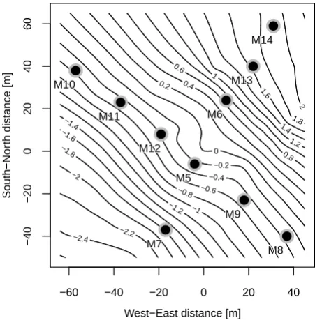
Fig. 1. Sampling locations for sub-canopy CO2concentration at a 2.25 m height. M-numbers are used for reference in the text. Topog-raphy is shown by isolines with an equidistance of 0.2 m relative to 750 m ASL.
2 Material and methods
2.1 Site 175
Measurements were carried out at the FLUXNET site Waldstein-Weidenbrunnen (DE-Bay), 50° 08’ 31”N, 11° 52’ 01”E, a hill site in the Fichtelgebirge Mountains in Southern
Germany. The Norway spruce (Picea abies) stand is on the
upper section of a forested hill, 775 m ASL, with a 3 ° slope
180
facing south-west. The tree height within the footprint of the measurements is 25 m. The site is described in detail in Ger-stberger et al. (2004) and a summary of background data can be found in Staudt and Foken (2007).
2.2 Instrumental setup 185
Wind vector and CO2 concentration time series were
recorded along horizontal transects at a 2.25 m height in the sub-canopy space. The spatial setup of sub-canopy
sam-ple locations is shown in Fig. 1. Ten CO2 concentration
sample points were distributed between an along slope
tran-190
sect from north-east to south-west (5 sample points) and an across slope transect from north-west to south-east (6 sample points), including one common point. Each point was sampled by an individual closed-path infrared gas an-alyzer. Instruments used were five LI-6262, one LI-6251
195
(LI-COR Biosciences Inc.), four BINOS (Leybold Heraeus
GmbH). In addition to CO2concentration measurements at a
2.25 m height, sample locations M5, M6, M7, M8, M9, M10
(see Fig. 1) were equipped with sonic anemometers (USA-1, METEK GmbH) to measure wind speed, wind direction
200
and sonic temperature at the same height. CO2
concentra-tion measurements are available with a frequency of 1 Hz at each sample point, sonic data were recorded at a 20 Hz frequency. To reduce the risk of systematic differences be-tween individual closed-path gas analyzers the system was
205
carefully designed to avoid any possible bias of the concen-tration measurement from differences in pressure or temper-ature (sample air tempertemper-ature, ambient analyzer tempertemper-ature,
radiation). All CO2closed-path gas analyzers shared a
com-mon housing in a central position with controlled conditions
210
resulting in a constant common temperature and common pressure regime. Moreover, all analyzers shared a common tailor-made automatic calibration system, using high
preci-sion reference gases (accuracy 0.1µmol mol−1). The
cal-ibration routine included an automatic calcal-ibration every 4
215
hours using two reference concentrations, which were sam-pled by all ten analyzers at the same time. In addition to factory calibration, each instrument’s polynomial calibration function was established on site, using multiple standards. The polynomial was checked before and during the
experi-220
ment.
Individual technical measures taken to avoid systematic inter-instrument bias include the following:
– The length of tubing connecting each sample point with
the corresponding gas analyzer was exactly 75 m for
ev-225
ery point. Sample tubes used were of polyethylene-aluminum composite structure, model DEKABON 1300-M060X (Serto AG, Fuldabr¨uck, Germany) with an inner diameter of 4 mm.
– Large diameter line intake air filters were checked
reg-230
ularly and replaced synchronously at all points, if nec-essary.
– Common ambient temperature and pressure for all gas
analyzers and calibration unit, including radiation pro-tection, active automatic temperature control by heating
235
and cooling as well as carefully designed ambient air circulation.
– Quality control of performance of automatic
tempera-ture control system, making sure that ambient air tem-peratures measured at several points surrounding the gas
240
analyzers remain within acceptable range.
– Temperature adaptation for sample lines, to allow the
temperature of sample air in all sample lines to equi-librate to a common temperature prior to entering the analyzer.
245
– Common temperature and radiation shielding for
refer-ence gases.
Fig. 1. Sampling locations for sub-canopy CO2concentration at a 2.25 m height. M-numbers are used for reference in the text. Topog-raphy is shown by isolines with an equidistance of 0.2 m relative to 750 m a.s.l.
2 Material and methods
2.1 Site
Measurements were carried out at the FLUXNET site Waldstein-Weidenbrunnen (DE-Bay), 50◦0803100N, 11◦5200100E, a hill site in the Fichtelgebirge Mountains in Southern Germany. The Norway spruce (Picea abies) stand is on the upper section of a forested hill, 775 m ASL, with a 3◦slope facing south-west. The tree height within the footprint of the measurements is 25 m. The site is described in detail in Gerstberger et al. (2004) and a summary of background data can be found in Staudt and Foken (2007).
2.2 Instrumental setup
Wind vector and CO2 concentration time series were recorded along horizontal transects at a 2.25 m height in the sub-canopy space. The spatial setup of sub-canopy sam-ple locations is shown in Fig. 1. Ten CO2 concentration sample points were distributed between an along slope tran-sect from north-east to south-west (5 sample points) and an across slope transect from north-west to south-east (6 sample points), including one common point. Each point was sampled by an individual closed-path infrared gas an-alyzer. Instruments used were five LI-6262, one LI-6251 (LI-COR Biosciences Inc.), four BINOS (Leybold Heraeus GmbH). In addition to CO2concentration measurements at a 2.25 m height, sample locations M5, M6, M7, M8, M9, M10
(see Fig. 1) were equipped with sonic anemometers (USA-1, METEK GmbH) to measure wind speed, wind direction and sonic temperature at the same height. CO2 concentra-tion measurements are available with a frequency of 1 Hz at each sample point, sonic data were recorded at a 20 Hz frequency. To reduce the risk of systematic differences be-tween individual closed-path gas analyzers the system was carefully designed to avoid any possible bias of the concen-tration measurement from differences in pressure or temper-ature (sample air tempertemper-ature, ambient analyzer tempertemper-ature, radiation). All CO2closed-path gas analyzers shared a com-mon housing in a central position with controlled conditions resulting in a constant common temperature and common pressure regime. Moreover, all analyzers shared a common tailor-made automatic calibration system, using high preci-sion reference gases (accuracy 0.1 µmol mol−1). The calibra-tion routine included an automatic calibracalibra-tion every 4 h using two reference concentrations, which were sampled by all ten analyzers at the same time. In addition to factory calibration, each instrument’s polynomial calibration function was estab-lished on site, using multiple standards. The polynomial was checked before and during the experiment.
Individual technical measures taken to avoid systematic inter-instrument bias include the following:
– The length of tubing connecting each sample point with
the corresponding gas analyzer was exactly 75 m for ev-ery point. Sample tubes used were of polyethylene-aluminum composite structure, model DEKABON 1300-M060X (Serto AG, Fuldabr¨uck, Germany) with an inner diameter of 4 mm.
– Large diameter line intake air filters were checked
reg-ularly and replaced synchronously at all points, if nec-essary.
– Common ambient temperature and pressure for all gas
analyzers and calibration unit, including radiation pro-tection, active automatic temperature control by heating and cooling as well as carefully designed ambient air circulation.
– Quality control of performance of automatic
tempera-ture control system, making sure that ambient air tem-peratures measured at several points surrounding the gas analyzers remain within acceptable range.
– Temperature adaptation for sample lines, to allow the
temperature of sample air in all sample lines to equi-librate to a common temperature prior to entering the analyzer.
– Common temperature and radiation shielding for
refer-ence gases.
– Minimization of dead volumes in calibration and valve
– Flow rate of 2 L min−1 (Reynolds number Re = 2520) above critical flow rate of 1.8 L min−1 at critical Reynolds number (Recrit=2320) to ensure turbulent flow conditions in all tubes, at the same time keeping the flow rate as low as possible to minimize pressure drop across the system.
– Regular flow rate check and adjustment for all sample
lines.
– Bypass system to avoid back pressure effects during
calibration, featuring a low pressure drop bypass flow rate control device to ensure minimum necessary by-pass flow and avoid possible reverse flow and sample contamination by ambient air.
– One common pump downstream of the analyzers to
re-duce effects of the pump on the concentration signals and to guarantee common pressure for all analyzers, as-suming equal pipe geometry of all sample lines.
– Automatic control of constant overall system flow rate
by mass flow controller.
– Passive system to allow for pressure equilibration
be-tween sample cells of individual gas analyzers by con-necting all analyzer outlets to a manifold with a suffi-ciently large diameter.
– Pre-assembly measurement and evaluation of the
pres-sure drop caused by individual system components to ensure that associated errors of the CO2 concentration measurements are below accepted threshold.
– Vacuum and over pressure assisted leak check for the
complete system to rule out sample contamination by ambient air.
2.3 Data set
The data set was collected during the second intensive obser-vation period (IOP2), 1 June to 15 July 2008 of the EGER (“ExchanGE processes in mountainous Regions”) experi-ment (Serafimovich et al., 2008). 24.6 days worth of data were used for the analysis, i.e. 1181 half hourly values taken from a window of 32.0 days (11 June to 13 July). Peri-ods were excluded from the analysis when instruments were powered off or obviously malfunctioning.
2.4 Theoretical considerations regarding concentration
differences
2.4.1 Bias
An observed concentration difference between two spatially separated sample points is the sum of a concentration dif-ference originating from a natural atmospheric concentration
gradient and the inter instrument bias, the latter being de-termined by systematic (bias) and random error of the indi-vidual instruments. We will refer to this composite concen-tration difference also as a concenconcen-tration offset,1c. While random error of the instruments is a minor concern in the current study due to sufficiently long averaging period, in-strument bias can be reduced by calibration against known standards. The calibration procedure used in this study was outlined in Sect. 2.2. The remaining bias is the sum of the error of the calibration plus the instrument drift between two consecutive calibration events. This remaining bias cannot be removed by calibration since it is intrinsic to the calibra-tion procedure itself. However, a statistical approach detailed in Sect. 2.7 can help to distinguish between remaining bias and concentration differences originating from natural gradi-ents based on the observed signal.
2.4.2 Natural concentration differences
To separate concentration differences originating from nat-ural gradients between two spatially disjunct (i.e. up to a few tens of meters) sample points from instrument bias the following assumption is made and is the basis for bias cor-rection used in the current study: for certain meteorologi-cal conditions the concentration time series observed simul-taneously at the two locations can be statistically linked to a reference concentration which is common to both sam-ple locations. To be more precise, under the condition of well mixed, i.e. sufficiently turbulent atmospheric conditions (hereafter “mixed” conditions) the concentration difference between the two locations which is most likely to be ob-served is zero. If this statement is true for the concentration difference between any two points, it can also be applied to the difference between the concentration at one sample loca-tionci, and the spatial average concentration of the sample
point fieldc(t )˜ at a given timet.c(t ), which serves as a refer-˜ ence concentration, describes the background concentration of the sample point field at timetusing the median field con-centration according to Eq. (1):
˜ c=
ck+1
2 kodd
1 2
ck
2
+ck
2+1
keven (1)
withk=1...nobservations(c1,c2,...,ck)being the
concen-tration measurements (c1(t ),c2(t ),...,cn(t )) at n locations
sorted in ascending order. The statistical measure describ-ing the concentration difference most likely to be observed is the mode of the probability density distribution (pdf) of the concentration differencesci(t )− ˜c(t ), which is assumed to
be close to zero under the condition of well mixed i.e. suffi-ciently turbulent atmospheric conditions.
2
L. Siebicke, G. Steinfeld and T. Foken: CO2gradient measurements using a parallel multi-analyzer setup 5
● ●
● ● ●
● ●
●
● ●
0 2 4 6 8 10
0
2
4
6
8
10
time
concentr
ation
● c1(t) c2(t)
(a)
concentration difference
Frequency
0
2
4
6
8
10
Density
0.0
0.2
0.4
0.6
0.8
1.0
−4 −2 0 2 4 c1(t)−c~(t) c2(t)−c~(t)
(b)
● ●
● ● ●
● ●
● ●
●
0 2 4 6 8 10
0
2
4
6
8
10
time
concentr
ation
● c1(t) c2(t)
(c)
concentration difference
Frequency
0
2
4
6
8
10
Density
0.0
0.2
0.4
0.6
0.8
1.0
−4 −2 0 2 4 c1(t)−c~(t) c2(t)−c~(t)
(d)
Fig. 2.Hypothetical concentration time seriesc1(t)andc2(t)with
timet∈[1,10](a,c), and corresponding frequency and density dis-tributions of concentration differencesci(t)−˜c(t)(b,d)for mixed
conditions (a,b) and for non mixed conditions (c,d). Regarding the density distributions in Subfig. (b) and (d), the histogram bars in-dicate the frequency for binwidths of 1.0, the solid line is a kernel density estimation generated with the same tools which were used for density estimation of measured concentration data as described in Sect. 2.7.
is themodeof the probability density distribution (pdf) of
the concentration differencesci(t)−˜c(t), which is assumed
to be close to zero under the condition of well mixed i.e.
suf-340
ficiently turbulent atmospheric conditions.
This is illustrated in Fig. 2(b) for two
hypotheti-cal time series c1(t) = 7,6,5,5,8,5,4,6,5,6 and c2(t) =
7,6,7,5,3,5,4,5,6,5, displayed in Fig. 2(a). The
characteris-tics of turbulence justify the assumedmodeof thepdf to be
345
close to zero, i.e. turbulence consists of temporal perturba-tions of a mean state which are stochastic and relatively short
in duration compared to the observation period. Themode
is zero even though the time seriesc1(t)andc2(t)given in
Fig. 2(a) have a different mean (temporal mean indicated by
350
overline): c1(t) = 5.7 andc2(t) = 5.3, and even though the
mean of the concentration differenceci(t)−˜c(t)is different
from zero:c1(t)−c˜(t) = 0.2andc2(t)−c˜(t) =−0.2.
For atmospheric conditions without turbulent mixing (hereafter “non mixed” conditions) above stated assumption
355
does not need to be fullfilled. Since there is no effective mechanism of mixing, two sample locations can be contin-uously exposed to air masses with different concentrations
– see concentration time seriesc1(t) = 4,3,2,2,5,2,1,3,2,3
andc2(t) = 8,7,8,6,4,6,5,6,7,6in Fig. 2(c) – i.e. there is a 360
persistent natural gradient and no common background con-centration is observed at both sample points. Thus, the two points will most frequently sample a concentration difference
which represents this gradient, and themodeof the
probabil-ity densprobabil-ity distribution is non zero, Fig. 2(d).
365
All combinations of the well mixed and non mixed case
are possible. It depends on turbulence statistics and the
length of the time series incorporated in the probability den-sity distribution whether mixing is sufficient to produce a
mode of thepdf close to zero or not. A method to
quan-370
tify the degree of mixing will be presented in Sect. 2.6.
2.5 Large Eddy Simulation
An idealized Large Eddy Simulation (LES) case study was performed in order to check whether the assumption made in Sec. 2.4.2 is true, i.e. whether the mode of the
proba-375
bility density function of the differenceci(t)−˜c(t)between
the scalar concentration at one sample locationci(t)and the
scalar concentration averaged over all sample pointsc˜(t)is
close to zero for well mixed conditions, even in the case that the distribution of sources and sinks of the scalar is not
homo-380
geneous and a mean spatial concentration gradient ∂y∂¯c with
concentrationcand horizontal distanceyexists. Large Eddy
Simulation is a tool that is used to study turbulence related processes in the atmospheric boundary layer. It can there-fore be used to extract statistical properties of turbulence for
385
the well mixed case. The simulation does not intend to per-fectly mimic subcanopy conditions but to test general statis-tical properties of turbulent mixing, i.e. whether strong tur-bulent mixing is able to allow the average field background
concentrationc˜(t)to emerge as the dominant mode of the
390
probability density function rather than local sources or sinks producing the dominant mode.
The LES model used in this study is the Parallelised LES Model (PALM) that has been developed at the Institute of Meteorology and Climatology at the Leibniz University in
395
Hannover, Germany. Detailed information on the LES ap-proach, model equations and numerical schemes applied in PALM are given in Raasch and Schr¨oter (2001) or – continu-ously updated – on-line on the homepage of the PALM group (Raasch, 2010). In our applications of PALM presented here
400
an additional prognostic equation for a scalar quantity was solved so that the temporal development of a scalar concen-tration field with distributed sources and sinks could be sim-ulated.
Two simulations with different setups were carried out for
405
this study. In our first simulation (“case A”) a horizontally
homogeneous distribution of scalar sourcesand sinkswas
prescribed. However, the scalar concentrationfieldwas
ini-tialized with a horizontal concentration gradient. This setup resulted in a temporally decaying horizontal concentration
410
gradient due to turbulent mixing.
Fig. 2. Hypothetical concentration time seriesc1(t )andc2(t )with timet∈ [1,10](a, c), and corresponding frequency and density dis-tributions of concentration differencesci(t )− ˜c(t )(b, d) for mixed
conditions (a, b) and for non mixed conditions (c, d). Regarding the density distributions in Fig. b and d, the histogram bars indicate the frequency for binwidths of 1.0, the solid line is a kernel density es-timation generated with the same tools which were used for density estimation of measured concentration data as described in Sect. 2.7.
close to zero, i.e. turbulence consists of temporal perturba-tions of a mean state which are stochastic and relatively short in duration compared to the observation period. The mode is zero even though the time seriesc1(t )andc2(t )given in Fig. 2a have a different mean (temporal mean indicated by overline): c1(t )=5.7 andc2(t )=5.3, and even though the mean of the concentration differenceci(t )− ˜c(t )is different
from zero:c1(t )− ˜c(t )=0.2 andc2(t )− ˜c(t )= −0.2. For atmospheric conditions without turbulent mixing (hereafter “non mixed” conditions) above stated assumption does not need to be fullfilled. Since there is no effective mechanism of mixing, two sample locations can be contin-uously exposed to air masses with different concentrations – see concentration time seriesc1(t )=4,3,2,2,5,2,1,3,2,3 andc2(t )=8,7,8,6,4,6,5,6,7,6 in Fig. 2c – i.e. there is a persistent natural gradient and no common background con-centration is observed at both sample points. Thus, the two points will most frequently sample a concentration difference which represents this gradient, and the mode of the probabil-ity densprobabil-ity distribution is non zero, Fig. 2d.
All combinations of the well mixed and non mixed case are possible. It depends on turbulence statistics and the
length of the time series incorporated in the probability den-sity distribution whether mixing is sufficient to produce a mode of the pdf close to zero or not. A method to quantify the degree of mixing will be presented in Sect. 2.6.
2.5 Large Eddy Simulation
An idealized Large Eddy Simulation (LES) case study was performed in order to check whether the assumption made in Sect. 2.4.2 is true, i.e. whether the mode of the proba-bility density function of the differenceci(t )− ˜c(t )between
the scalar concentration at one sample locationci(t )and the
scalar concentration averaged over all sample pointsc(t )˜ is close to zero for well mixed conditions, even in the case that the distribution of sources and sinks of the scalar is not homo-geneous and a mean spatial concentration gradient ∂∂yc¯ with concentrationcand horizontal distanceyexists. Large Eddy Simulation is a tool that is used to study turbulence related processes in the atmospheric boundary layer. It can there-fore be used to extract statistical properties of turbulence for the well mixed case. The simulation does not intend to per-fectly mimic subcanopy conditions but to test general statis-tical properties of turbulent mixing, i.e. whether strong tur-bulent mixing is able to allow the average field background concentration c(t )˜ to emerge as the dominant mode of the probability density function rather than local sources or sinks producing the dominant mode.
The LES model used in this study is the Parallelised LES Model (PALM) that has been developed at the Institute of Meteorology and Climatology at the Leibniz University in Hannover, Germany. Detailed information on the LES ap-proach, model equations and numerical schemes applied in PALM are given in Raasch and Schr¨oter (2001) or – continu-ously updated – on-line on the homepage of the PALM group (Raasch, 2010). In our applications of PALM presented here an additional prognostic equation for a scalar quantity was solved so that the temporal development of a scalar con-centration field with distributed sources and sinks could be simulated.
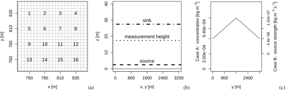
Two simulations with different setups were carried out for this study. In our first simulation (“case A”) a horizontally homogeneous distribution of scalar sources and sinks was prescribed. However, the scalar concentration field was ini-tialized with a horizontal concentration gradient. This setup resulted in a temporally decaying horizontal concentration gradient due to turbulent mixing.
In the second simulation (“case B”) the initial field of scalar concentration and the sinks of scalar concentration were prescribed to be horizontally homogeneous. However, the sources of scalar concentration were horizontally hetero-geneously distributed. This setup resulted in a temporally evolving concentration gradient.
x [m]
y [m]
760 785 810 835
760
785
810
835 1 2 3 4
5 6 7 8
9 10 11 12
13 14 15 16
(a)
0
10
20
30
40
x, y [m]
z [m]
sink
measurement height
source
0 800 1600 2400 3200
(b) y [m]
Case A: concentr
ation [kg
m
−
3]
0 800 2400
0
3.50e−04
9.40e−04
Case B: source strength [
k
g
m
−
3s
−
1]
0
4.4e−08
1.32e−07
(c)
Fig. 3. Setup of Large Eddy Simulation study. Virtual sensor locations (a), Source-sink distribution (b) and background concentration gradient (c). Grid spacing: 5 m.
common to both simulations will be reported before pointing out details regarding the scalar concentration field which are specific to each setup.
In both simulations the model domain consisted of 640×640×256 grid points and a basic grid spacing of 5 m was used. Above a height of 1000 m the grid was stretched vertically until a maximum grid size of 20 m was reached. The total extension of the model domain was 3.2×3.2×2 km.
Both LES simulations were initialized with wind profiles that were obtained from a one-dimensional prerun in order to accelerate the transition to a stationary state in the three-dimensional main run. The geostrophic wind (ug, vg) was
prescribed as (3 m s−1, 0 m s−1) whileuandvcorrespond to thex- andy-direction, respectively. The roughness length was 0.1 m. At the bottom boundary of the model domain a near-surface heat flux of 0.01 K m s−1was prescribed, so that a convective boundary layer with an Obukhov-length in the range between−40 and −50 m developed with time. The Coriolis parameter corresponded to a geographical latitude of 55◦.
Sources and sinks of the scalar were switched on as soon as the simulation had reached a quasi-stationary state, i.e. after a spin-up time of 2 h. The sources of the scalar were situated at a height of 2.5 m and distributed homogeneously over the total horizontal extension of the model domain. The sinks of the scalar were also distributed over the total hori-zontal extension of the model domain but situated at a height of 27.5 m.
In both simulations time series of scalar concentration were recorded at 16 observation points within thexy-cross section of the model domain at a height of 17.5 m beginning from the first release of scalar quantity until the end of the LES 7200 s later. Data from these time series could be used in order to calculate the differences between the concentra-tion at a single sample point and the concentraconcentra-tion averaged over all sample points as required in order to check the
va-lidity of the assumption made in Sect. 2.4.2. Figure 3 shows the locations of these observation points of the two LES. The coordinates of the 16 observation points were composed out of the x-coordinates (760 m, 785 m, 810 m, 835 m) and y-coordinates (760 m, 785 m, 810 m, 835 m). Thus, the dis-tance between two adjacent observation points along the x-ory-direction was 25 m.
In case A the initial scalar concentration field showed a gradient along they-direction. The initial concentration in-creased by 3.038×10⁻⁷kg m−4fromy=0 toy=Ly
2, while it decreased by 3.038×10⁻⁷kg m−4fromy=Ly
2 toy=Ly (Lyis the length of the model domain along they-direction).
It is worth mentioning that the prescribed gradients are equiv-alent to±0.16µmol mol−1m−1which deliberately has been chosen to represent the maximum of gradients observed in the field at the site under study and published for other sites (Aubinet et al., 2003; Heinesch et al., 2007) during stable stratification, even though gradients are smaller during neu-tral and unstable stratification, i.e. the stratification regime present in the LES. In that sense, the LES with strong gradi-ents tests a worst case scenario.
As in case B the initial mean scalar concentration prior to imposing the additional spatial gradients in case A was 6.997×10⁻⁴kg m−3. Note that this is equiva-lent to 378 µmol mol−1 CO2, which was the background concentration observed at the experimental test site de-scribed in Sect. 2.1. The resulting initial concentration field is shown in Fig. 3c. The source strength was set to 8.8×10⁻⁸kg m−3s−1, while the sink had a strength of −8.8×10⁻⁸kg m−3s−1. It was chosen to correspond to a typical maximum daytime Net Ecosystem Exchange of −20 µmol m−2s−1observed at the measurement site.
In case B (horizontally homogeneous initial concentra-tion field) a basic source strength of 4.4×10⁻⁸kg m−3s−1 was prescribed at y=0 and y =Ly. Between y=0
and y = Ly
2 the gradient of the source strength,
2
was 5.5×10⁻¹¹kg m−4s−1 for y < Ly
2, while it was −5.5×10⁻¹¹kg m−4s−1 between y = Ly
2 and y =Ly. Thus, the mean horizontal source strength was exactly the same as in case A. The sink strength was prescribed as in case A (and thus again approx. equivalent to a typical maximum daytime Net Ecosystem Exchange of−20 µmol m−2s−1 ob-served at the site).
It is obvious that the Large Eddy Simulations presented here are an idealization and do not account for the complex-ity of the given forest site, particularly because they do not fully account for the forest canopy. However, we would like to stress that the purpose of the simulation is to test the ide-alized case of turbulent mixing given realistic physical val-ues of scalar concentration gradients and a vertical source and sink distribution that does mimic sources at the forest floor and sinks in the forest canopy with respect to their ver-tical distribution and their intensity. Verifying and accepting the assumption made in Sect. 2.4.2 first for an idealized case is necessary before addressing measurements from the more complex forest setting. Whether conditions in the forest at any given time show sufficient mixing is not evaluated by LES but by the application of an empirical mixing index (see Sect. 2.6) which is based on measured data.
2.6 Mixing index
A “mixing index” MI was formulated to quantify the de-gree of mixing between the real world sample points given in Fig. 1. A threshold value MIc was then used to sepa-rate well mixed conditions from not sufficiently mixed con-ditions. The mixing index MI was based on cross correlation R(τ ), e.g.Rc1c2(τ ) of the simultaneous concentration time
seriesc1(t )andc2(t )at spatially separated sample locations, normalized by their mean varianceσ2. The cross correlation function is given as:
Rc1c2(τ )=
1 TF
Z TF/2
−TF/2
c1(t )·c2(t+τ )dt (2)
with time lagτ between concentration time seriesc1(t )and c2(t ),TF being the length of the time window ofc1(t )and c2(t )andτ∈ [−TF,TF]. MI then writes:
MI=max(|Rc1c2(τ )|)·
σc2
1+σ
2
c2
2 !−1
. (3)
More specifically, MI was calculated using the mean cross correlation of CO2 concentration time series c5 and c6recorded at a sample point pair oriented along the terrain slope (locations M5, M6) andc5andc8recorded at a sam-ple point pair oriented across the slope (M5, M8) divided by the mean field variance of all concentration time series c5,c6,...,c14 at sample locations M5,M6,...,M14 using a window length ofTF=60 min.
2
In case B (horizontally homogeneous initial
concentra-tion field) a basic source strength of4.4×10−8kg m−3s−1
was prescribed at y= 0 and y =Ly. Between y= 0
490
and y = Ly
2 the gradient of the source strength,
∂s ∂y,
was 5.5×10⁻¹¹kg m−4s−1 for y < Ly
2 , while it was
−5.5×10⁻¹¹kg m−4s−1 between y= Ly
2 and y =Ly.
Thus, the mean horizontal source strength was exactly the same as in case A. The sink strength was prescribed as in
495
case A (and thus again approx. equivalent to a typical
maxi-mum daytime Net Ecosystem Exchange of -20µmol m−2s−1
observed at the site).
It is obvious that the Large Eddy Simulations presented here are an idealization and do not account for the
complex-500
ity of the given forest site, particularly because they do not fully account for the forest canopy. However, we would like to stress that the purpose of the simulation is to test the ide-alized case of turbulent mixing given realistic physical val-ues of scalar concentration gradients and a vertical source
505
and sink distribution that does mimic sources at the forest floor and sinks in the forest canopy with respect to their ver-tical distribution and their intensity. Verifying and accepting the assumption made in Sec. 2.4.2 first for an idealized case is necessary before addressing measurements from the more
510
complex forest setting. Whether conditions in the forest at any given time show sufficient mixing is not evaluated by LES but by the application of an empirical mixing index (see Sec. 2.6) which is based on measured data.
2.6 Mixing index 515
A “mixing index” MI was formulated to quantify the
de-gree of mixing between the real world sample points given
in Fig. 1. A threshold value MIc was then used to
sepa-rate well mixed conditions from not sufficiently mixed
con-ditions. The mixing indexMIwas based on cross correlation
520
R(τ), e.g. Rc1c2(τ)of the simultaneous concentration time
seriesc1(t)andc2(t)at spatially separated sample locations,
normalized by their mean varianceσ2. The cross correlation
function is given as:
Rc1c2(τ) =
1
TF
Z TF/2
−TF/2
c1(t)·c2(t+τ)dt (2) 525
with time lagτ between concentration time seriesc1(t)and
c2(t),TF being the length of the time window ofc1(t)and
c2(t)andτ∈[−TF,TF].MIthen writes:
M I= max(|Rc1c2(τ)|)· σ2
c1+σ
2
c2
2
−1
. (3)
More specifically, MI was calculated using the mean cross
530
correlation of CO2 concentration time series c5 and c6
recorded at a sample point pair oriented along the terrain
slope (locations M5, M6) andc5andc8recorded at a
sam-ple point pair oriented across the slope (M5, M8) divided
0.0 0.2 0.4 0.6
0
2
4
6
8
10
12
Mixing index MI
Density
(a)
● ●●●● ● ●
● ●
●
● ●
● ●
●
●
●
●● ● ●● ●●
Time, CET
Mixing inde
x MI
00:00 12:00 24:00
0.00
0.10
0.20
0.30
(b)
Fig. 4.Density distribution of mixing indexMI(solid line). Dashed lines atMI=0.06 andMI=0.12 enclose range for sensible choices of a critical mixing indexMIc,(a). Diurnal course of mixing index on 29 June 2008 (solid line) andMIc(dashed line),(b). MIis repre-sentative for the whole sample point field (see Sect. 2.6 for details of the calculation).
by the mean field variance of all concentration time series
535
c5,c6,...,c14 at sample locations M5,M6,...,M14 using a
window length ofTF=60 min. The critical mixing index
MIcwas empirically inferred from the density distribution of
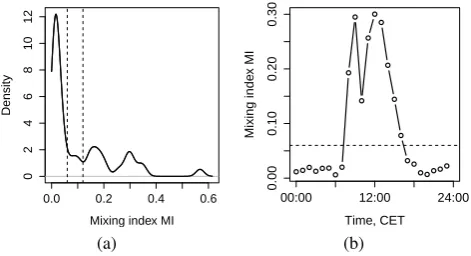
MI given in Fig. 4(a). Sensible values were found to be in
the rangeMIc∈[0.06,0.12], corresponding to a sharp bend
540
in the density distribution separatingMI’s representative of
well mixed daytime conditions (distribution tail to the right
ofMIcin Fig. 4a) from lowMI’s representative of night time
conditions with little mixing (distribution peak to the left of
MIcin Fig. 4a). Figure 4b presents a typical diurnal cycle of
545
the mixing index which is clearly separated into mixed and
non mixed conditions byMIc.
2.7 Bias correction
A statistical correction was applied to the CO2
concentra-tion time series ci(t) of every individual analyzer (which
550
had previously been calibrated against known reference gas standards) to correct for remaining instrument related bias
∆ci. This yields the statistically bias corrected time series
ci,corr(t)according to Eq. (4):
ci,corr(t) =ci(t)−∆ci for M I≥M Ic (4)
555
Instrument related bias of the CO2 concentration signal
was observed to vary over time. It is therefore appropriate to apply a bias correction that is time dependent, too. Analyzer
specific values of instrument bias∆ciwere computed for
ev-ery 60-minute intervalTF of the concentration time series
560
ci(t)by finding themode(max(density)) of the probability
density distribution (pdf) of the instantaneous concentration
differences of an individual analyzerci(t)relative to the field
average concentrationc˜(t)according to:
∆ci= max(pdf (ci(t)−c˜(t))) (5)
565
Fig. 4. Density distribution of mixing index MI (solid line). Dashed lines at MI = 0.06 and MI = 0.12 enclose range for sensible choices of a critical mixing index MIc, (a). Diurnal course of mixing index on 29 June 2008 (solid line) and MIc(dashed line), (b). MI is rep-resentative for the whole sample point field (see Sect. 2.6 for details of the calculation).
The critical mixing index MIc was empirically inferred from the density distribution of MI given in Fig. 4a. Sen-sible values were found to be in the range MIc∈ [0.06,0.12], corresponding to a sharp bend in the density distribution sep-arating MI’s representative of well mixed daytime conditions (distribution tail to the right of MIc in Fig. 4a) from low MI’s representative of night time conditions with little mix-ing (distribution peak to the left of MIcin Fig. 4a). Figure 4b presents a typical diurnal cycle of the mixing index which is clearly separated into mixed and non mixed conditions by MIc.
2.7 Bias correction
A statistical correction was applied to the CO2 concentra-tion time seriesci(t )of every individual analyzer (which had
previously been calibrated against known reference gas stan-dards) to correct for remaining instrument related bias1ci.
This yields the statistically bias corrected time seriesci,corr(t ) according to Eq. (4):
ci,corr(t )=ci(t )−1ci for MI≥MIc (4) Instrument related bias of the CO2concentration signal was observed to vary over time. It is therefore appropriate to ap-ply a bias correction that is time dependent, too. Analyzer specific values of instrument bias 1ci were computed for
every 60-minute intervalTF of the concentration time series ci(t )by finding the mode (max(density)) of the probability
density distribution (pdf) of the instantaneous concentration differences of an individual analyzerci(t )relative to the field
average concentrationc(t )˜ according to:
1ci=max(pdf(ci(t )− ˜c(t ))) (5)
Identifying the mode of the pdf requires a robust estimate of the distribution. A comparison of histogram based and kernel-density-estimator based approaches showed that the latter are superior in terms of robustness relative to scatter in the distribution, which is a valuable feature particularly for limited sample sizes. Density estimates were generated using a moving window Gaussian kernel for smoothing (Wand and Jones, 1995). The optimal width of the window was adap-tively and automatically found using pilot-density-estimates according to Sheather and Jones (1991), implemented in the dpik function of the KernSmooth library (Ripley, 2009) vided with R (R Development Core Team, 2009), also pro-viding the bkde function which was used to estimate the density.
Having found an individual bias value for every analyzer, the mixing index was checked to decide whether concentra-tion time series correcconcentra-tion was applicable. For well mixed conditions, i.e. MI≥MIc, the observed 60-minute concentra-tion time seriesci(t )of every analyzer was shifted by the
an-alyzer specific bias value1ci found for the given 60-minute
interval, yielding the bias corrected concentration time se-riesci,corr(t )according to Eq. (4). For MI<MIc the cor-rection was applied using the last valid bias value satisfying MI≥MIc.
In order to verify that concentration offsets1ci found are
related to slow drift of the analyzers (instrument bias) rather than driven by meteorological forcing of natural concentra-tion gradients, a regression analysis was performed studying the correlation of1ci versus ambient air temperature,
pres-sure and atmospheric stability ζ, respectively. The stabil-ity parameterζ is defined asζ =(z−d)L−1with measure-ment heightz, displacement heightdand Obukhov-lengthL. No significant correlation was found between the concentra-tion offset and the three meteorological parameters, which is an indication that the calculated offset1ci is dominated
by instrument bias and should therefore be removed with the proposed conditional bias correction approach, respect-ing MI≥MIc.
Because, even under mixed conditions, natural concentra-tion differences could account for a (very small) part of the observed concentration offsets 1ci, an error analysis was
performed. The aim was to quantify the benefit of the ap-plication of the bias correction approach in a hypothetical “worst case” scenario, i.e. assuming that observed concentra-tion offsets1ci are solely determined by natural
concentra-tion differences rather than instrument bias. A relative error is defined in Eq. (6), describing the ratio of the error possi-bly attributed to the bias correction approach to the improve-ment achieved by the correction, which can be expressed as the span of the range of instrument bias (“drift span”). This relative error writes:
errorrel=Q1(1offi)−Q4(1offi) max(offi)−min(offi)
(6) with the change of the concentration offset1cibetween two
consecutive 60-minute intervals 1offi =1ci(t )−1ci(t−
60 min)and with Q1and Q4being the 25% and 75% quar-tiles of the density distribution, respectively, which reflect a typical range of1offi.
2.8 Net ecosystem exchange and horizontal advection
This section indicates the relevance of measurements of CO2 concentration gradients for the quantification of the exchange of CO2across the vegetation-atmosphere interface, i.e. the Net Ecosystem Exchange of CO2 (NEE). NEE can be cal-culated according to the following formula (Aubinet et al., 2003; Feigenwinter et al., 2004, and others):
NEE= 1 Vm
h Z
0 ∂c
∂t
dz+ 1 Vm
w0c0
h
+ 1 Vm
h Z
0
w(z)∂c ∂z+c(z)
∂w ∂z
dz
+ 1 Vm
h Z
0
u(z)∂c ∂x+v(z)
∂c ∂y
dz (7)
with the molar volume of dry air Vm, CO2 concentration c, time t, horizontal distances x and y, vertical distance above groundz, height of the control volumeh, horizontal wind velocity ualong the x-direction, horizontal wind ve-locityv along they-direction and vertical wind velocityw along thez-direction. Over-bars denote temporal means and primes denote the temporal fluctuations relative to the tempo-ral mean. The terms on the right hand side of Eq. (7) are the change of storage (term I), the vertical turbulent flux (term II), vertical advection (term IIIa), vertical mass flow from the surface e.g. due to evaporation (term IIIb) according to Webb et al. (1980), and horizontal advection (term IV). The form of NEE presented in Eq. (7) excludes the horizontal variation of the vertical turbulent flux and the horizontal variation of ver-tical advection. Eq. (7) further neglects the flux divergence term: Vm1
h R
0
∂
u0c0
∂x + ∂
v0c0
∂y !
dz. Term II and sometimes
terms I and III on the right hand side of Eq. (7) are central components of routine flux measurements at many sites and will not be discussed here. In contrast, term IV, the observa-tion of which is challenging and has only been realized in a limited number of experiments, shall be addressed here.
Accurate observations of horizontal concentration gradi-ents of CO2are important for the determination of horizontal advectionFHA, becauseFHA is the product of the horizon-tal wind velocity and the horizonhorizon-tal concentration gradient of the scalar CO2according to Eq. (8):
FHA= 1 Vm
h Z
0
¯ u(z)∂c¯
∂x+ ¯v(z) ∂c¯ ∂y
2
The fact that density distributions of concentration differ-ences can have a mode of zero and a non zero mean, as seen in Fig. 5b, is a crucial feature for the computation of horizon-tal advection, because only a non zero mean gradient∂x∂c¯6=0 and/or ∂y∂c¯6=0 can generate a non zero horizontal advection termFHA.
3 Results
After presenting results of the LES study, which contribute to the acceptance of the assumptions stated in Sect. 2.4.2, this section subsequently presents results of measured CO2 con-centration time series and gradients before and after applying the conditional bias correction as well as statistics about the improvement which can be achieved by the correction. Fur-thermore, observed concentration differences are put in the context of atmospheric stratification.
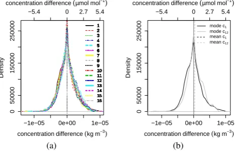
The results of the LES study demonstrate that for the given simulation the assumption stated in Sect. 2.4.2 is valid, i.e. the mode of the density distribution of the concentration dif-ference between any sample point and the sample point field average is essentially zero, Fig. 5a. Since both case A and case B lead to the same conclusion, only data of case B are shown in Fig. 5. Observed deviations of the density distri-bution mode from zero are insignificant, with the maximum deviation, considering all instrument’s distributions, divided by the mean distance of the sample point from the sample point field center, accounting for a 2.0% fraction only of the prescribed concentration gradient in the LES (case A). For case B the maximum deviations of the mode from zero were +0.015 and−0.025 µmol mol−1. Dividing this range of dis-tribution modes by the range of the disdis-tributions means yields a fraction of 0.15. Considering the small gradients under well mixed conditions, this is a very small error. Conditions with large gradients are not an issue because they are excluded by the mixing index filter and are not used to determine concen-tration offsets when applying the bias correction approach.
The given deviations of the pdf’s modes translate to an error attributed to estimates of the horizontal advective flux component, if estimates are based on concentration measure-ments corrected using the bias correction approach and thus removing the small deviation of the mode from zero. This potential error in the advection estimate is small compared to other uncertainties typically associated with advection esti-mates, e.g. due to an insufficient number of sampling points in space such as the often limited number of observation height levels of horizontal gradients.
An important feature of the density distributions shown is their skewness, separating mode and mean of a given distri-bution as illustrated in Fig. 5b for two selected sample points. The difference in the mean values of the density distributions is due to the concentration gradient and source-sink distri-bution prescribed in the LES. It thus demonstrates that it is possible to compute advective flux terms even from
distri-L. Siebicke, G. Steinfeld and T. Foken: CO2gradient measurements using a parallel multi-analyzer setup 9
the scalar CO2according to Eq. (8):
FHA=
1 Vm h Z 0 ¯
u(z)∂¯c
∂x+ ¯v(z) ∂¯c ∂y
dz. (8)
The fact that density distributions of concentration
differ-ences can have a mode of zero and a non zero mean, as
seen in Fig. 5(b), is a crucial feature for the computation of
665
horizontal advection, because only a non zero mean
gradi-ent ∂x∂c¯6= 0and/or ∂y∂¯c6= 0can generate a non zero horizontal
advection termFHA.
3 Results
After presenting results of the LES study, which contribute to
670
the acceptance of the assumptions stated in Sect. 2.4.2, this
section subsequently presents results of measured CO2
con-centration time series and gradients before and after applying the conditional bias correction as well as statistics about the improvement which can be achieved by the correction.
Fur-675
thermore, observed concentration differences are put in the context of atmospheric stratification.
The results of the LES study demonstrate that for the given simulation the assumption stated in Sect. 2.4.2 is valid, i.e.
themodeof the density distribution of the concentration
dif-680
ference between any sample point and the sample point field average is essentially zero, Fig. 5(a). Since both case A and case B lead to the same conclusion, only data of case B are shown in Fig. 5. Observed deviations of the density
distri-butionmodefrom zero are insignificant, with the maximum
685
deviation, considering all instrument’s distributions, divided by the mean distance of the sample point from the sample point field center, accounting for a 2.0 % fraction only of the prescribed concentration gradient in the LES (case A). For case B the maximum deviations of the mode from zero were
690
+0.015 and -0.025µmolmol−1. Dividing this range of
distri-bution modes by the range of the distridistri-butions means yields a fraction of 0.15. Considering the small gradients under well mixed conditions, this is a very small error. Conditions with large gradients are not an issue because they are excluded by
695
the mixing index filter and are not used to determine concen-tration offsets when applying the bias correction approach.
The given deviations of the pdf’smodes translate to an
error attributed to estimates of the horizontal advective flux component, if estimates are based on concentration
measure-700
ments corrected using the bias correction approach and thus
removing the small deviation of the modefrom zero. This
potential error in the advection estimate is small compared to other uncertainties typically associated with advection esti-mates, e.g. due to an insufficient number of sampling points
705
in space such as the often limited number of observation height levels of horizontal gradients.
An important feature of the density distributions shown is
their skewness, separating mode and mean of a given
dis-−1e−05 0e+00 1e−05
0
50000
150000
250000
concentration difference (kg m−3)
Density 1 2 3 4 5 6 7 8 9 10 11 12 13 14 15 16 1 2 3 4 5 6 7 8 9 10 11 12 13 14 15 16 1 2 3 4 5 6 7 8 9 10 11 12 13 14 15 16 1 2 3 4 5 6 7 8 9 10 11 12 13 14 15 16 1 2 3 4 5 6 7 8 9 10 11 12 13 14 15 16 1 2 3 4 5 6 7 8 9 10 11 12 13 14 15 16 1 2 3 4 5 6 7 8 9 10 11 12 13 14 15 16 1 2 3 4 5 6 7 8 9 10 11 12 13 14 15 16 1 2 3 4 5 6 7 8 9 10 11 12 13 14 15 16 1 2 3 4 5 6 7 8 9 10 11 12 13 14 15 16 1 2 3 4 5 6 7 8 9 10 11 12 13 14 15 16 1 2 3 4 5 6 7 8 9 10 11 12 13 14 15 16 1 2 3 4 5 6 7 8 9 10 11 12 13 14 15 16 1 2 3 4 5 6 7 8 9 10 11 12 13 14 15 16 1 2 3 4 5 6 7 8 9 10 11 12 13 14 15 16 −5.4 0 2.7 5.4 concentration difference (µmol mol−1)
(a)
−1e−05 0e+00 1e−05
0
50000
150000
250000
concentration difference (kg m−3)
Density
mode c1 mode c12 mean c1 mean c12 −5.4 0 2.7 5.4 concentration difference (µmol mol−1)
(b)
Fig. 5. Density distribution of LES modelled concentration dif-ferences ci(t)−˜c(t) of a point measurement ci(t) relative to
the field average concentration˜c(t) for concentration time series c1(t),c2(t),...,c16(t)andn= 16sensor locations1,2,...,16(a),
and for c1(t) and c12(t)at sensor locations 1 and 12(b). Note
that the density distributions ofc1(t)−˜c(t)andc12(t)−c˜(t)have
a commonmodebut different mean.
tribution as illustrated in Fig. 5(b) for two selected sample
710
points. The difference in the mean values of the density dis-tributions is due to the concentration gradient and source-sink distribution prescribed in the LES. It thus demonstrates that it is possible to compute advective flux terms even from
distributions withmodeequal to zero, since the mean
gradi-715
ent, which is necessary to computeFHAaccording to Eq. (8),
is expressed in the mean which does not need to be zero even
though themodeis essentially zero.
In order to evaluate the performance of the bias
correc-tion, Fig. 6(a) shows the CO2 concentration evolution
dur-720
ing one day measured at ten locations in the sub-canopy on 29 June 2008 without bias correction but including cal-ibration using known reference gas standards. Figure 6(b) presents the same data after applying the bias correction. The comparison of the two figures clearly demonstrates that the
725
bias correction is able to remove systematic concentration offsets between different analyzers in the uncorrected mea-surements (Fig. 6a). The offsets are most obvious during well mixed daytime conditions – when natural concentration dif-ferences are relatively small – and could be eliminated
suc-730
cessfully in the bias corrected time series at all times of the day (Fig. 6b).
Inter-instrument bias leads to relatively constant offsets
between individual concentration measurements ci(t)
dur-ing daytime conditions (Fig. 6a), exactly matchdur-ing the
pe-735
riod of a high mixing index (Fig. 4b). The minor importance of concentration differences due to natural gradients during well mixed conditions is the reason why inter-instrument bias becomes the prominent component of observed inter-instrument concentration differences (compare also Fig. 9
740
and Fig. 10). Well mixed conditions with MI ≥ MIc and
Fig. 5. Density distribution of LES modelled concentration dif-ferences ci(t )− ˜c(t ) of a point measurement ci(t ) relative to
the field average concentrationc(t )˜ for concentration time series
c1(t ),c2(t ),...,c16(t )andn=16 sensor locations 1,2,...,16 (a), and for c1(t )and c12(t )at sensor locations 1 and 12 (b). Note that the density distributions ofc1(t )− ˜c(t )andc12(t )− ˜c(t )have a common mode but different mean.
butions with mode equal to zero, since the mean gradient, which is necessary to computeFHAaccording to Eq. (8), is expressed in the mean which does not need to be zero even though the mode is essentially zero.
In order to evaluate the performance of the bias correc-tion, Fig. 6a shows the CO2 concentration evolution dur-ing one day measured at ten locations in the sub-canopy on 29 June 2008 without bias correction but including calibra-tion using known reference gas standards. Figure 6b presents the same data after applying the bias correction. The com-parison of the two figures clearly demonstrates that the bias correction is able to remove systematic concentration offsets between different analyzers in the uncorrected measurements (Fig. 6a). The offsets are most obvious during well mixed daytime conditions – when natural concentration differences are relatively small – and could be eliminated successfully in the bias corrected time series at all times of the day (Fig. 6b). Inter-instrument bias leads to relatively constant offsets between individual concentration measurements ci(t )
![Fig. 2. Hypothetical concentration time seriestimeFig. 2. c 1 ( t ) and c 2 ( t ) withtime t ∈[ 1 , 1 0 ] (a,c), and corresponding frequency and density dis-tributions of concentration differences c i ( t ) −c˜ ( t ) (b,d) for mixedconditions (a,b) and for](https://thumb-us.123doks.com/thumbv2/123dok_us/223738.1515760/5.595.49.287.61.318/hypothetical-concentration-seriestimefig-corresponding-tributions-concentration-differences-mixedconditions.webp)