Construction of gene regulatory networks using biclustering and bayesian networks

R E S E A R C H

Open Access

Construction of Gene Regulatory Networks using

biclustering and Bayesian networks

Fadhl M Alakwaa

, Nahed H Solouma

and Yasser M Kadah

* Correspondence: fadlwork@gmail. com

1_{University of Science and} Technology, Sana’a, Yemen Full list of author information is available at the end of the article

Abstract

Background:Understanding gene interactions in complex living systems can be

seen as the ultimate goal of the systems biology revolution. Hence, to elucidate disease ontology fully and to reduce the cost of drug development, gene regulatory networks (GRNs) have to be constructed. During the last decade, many GRN

inference algorithms based on genome-wide data have been developed to unravel the complexity of gene regulation. Time series transcriptomic data measured by genome-wide DNA microarrays are traditionally used for GRN modelling. One of the major problems with microarrays is that a dataset consists of relatively few time points with respect to the large number of genes. Dimensionality is one of the interesting problems in GRN modelling.

Results:In this paper, we develop a biclustering function enrichment analysis toolbox (BicAT-plus) to study the effect of biclustering in reducing data dimensions. The network generated from our system was validated via available interaction databases and was compared with previous methods. The results revealed the performance of our proposed method.

Conclusions:Because of the sparse nature of GRNs, the results of biclustering techniques differ significantly from those of previous methods.

Background

The major goal of systems biology is to reveal how genes and their products interact to regulate cellular process. To achieve this goal it is necessary to reconstruct gene regu-latory networks (GRN), which help us to understand the working mechanisms of the cell in patho-physiological conditions. The structure of a GRN can be described as a wiring diagram that (1) shows direct and indirect influences on the expression of a gene and (2) describes which other genes can be regulated by the translated protein or transcribed RNA product of such a gene [1].

The local topology of a GRN has been used to predict various systems-level pheno-types. For instance, Dyer et al. [2] recently analyzed the intraspecies network of Pro-tein-Protein Interactions (PPIs) among the 1,233 unique human proteins spanned by host-pathogen PPIs. They found that both viral and bacterial pathogens tend to inter-act with hubs (proteins with many interinter-acting partners) and bottlenecks (proteins that are central to many paths in the network) in the human PPI network.

Within the last few years, a number of sophisticated approaches to the reverse engi-neering of cellular networks from gene expression data have emerged. These include

Boolean networks [3], Bayesian networks [4], association networks [5], linear models [6], and differential equations [7]. The reconstruction of gene networks is in general complicated by the high dimensionality of high-throughput data; i.e. a dataset consists of relatively few time points with respect to a large number of genes. In this study we develop a biclustering function enrichment analysis toolbox (BicAT-plus) to study the effect of biclustering in reducing data dimension.

Clustering algorithms [8-10] have been used to reduce data dimension, on the basis that genes showing similar expression patterns can be assumed to be co-regulated or part of the same regulatory pathway. Unfortunately, this is not always true. Two limita-tions obstruct the use of clustering algorithms with microarray data. First, all condi-tions are given equal weights in the computation of gene similarity; in fact, most conditions do not contribute information but instead increase the amount of back-ground noise. Second, each gene is assigned to a single cluster, whereas in fact genes may participate in several functions and should thus be included in several clusters [11].

A new modified clustering approach to uncovering processes that are active over some but not all samples has emerged, which is called biclustering. A bicluster is defined as a subset of genes that exhibit compatible expression patterns over a subset of conditions [12]. During the last ten years, many biclustering algorithms have been proposed (see [13] for a survey), but the important questions are: which algorithm is better? And do some algorithms have advantages over others?

Generally, comparing different biclustering algorithms is not straightforward as they differ in strategy, approach, time complexity, number of parameters and predictive capacity. They are strongly influenced by user-selected parameter values. For these rea-sons, the quality of biclustering results is also often considered more important than the required computation time. Although some comparative analytical studies have evaluated the traditional clustering algorithms [14-16], no such extensive comparison exists for biclustering even after initial trials have been made [12]. Ultimately, biologi-cal merit is the main criterion for evaluation and comparison among the various biclustering methods.

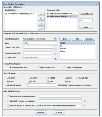
To the best of our knowledge, the biclustering algorithm comparison toolbox has not been made available in the literature. We have developed a comparative tool, BicAT-Plus (Figure 1), that includes comparative biological methodology and is to be used as an extension to the BicAT program [17]. BicAT-Plus and its manual can be down-loaded from these two links: http://home.k-space.org/BicAT-plus.zip and http://home. k-space.org/Bicat-plus-manual.pdf. BicAT is a java biclustering toolbox that contains five biclustering and two traditional clustering algorithms.

In this work, one of our goals was to study the value of biclustering algorithms for constructing GRNs.

Methods Data Acquisition

Two well-known datasets of yeast microarray gene expression (Gasch et al. [19]; Spell-man et al. [20]) were used in this work; they can downloaded from the Stanford Microarray Database (http://smd.stanford.edu/). The Spellman dataset consists of four synchronization experiments (alpha factor arrest, elutriation and arrest of CDC15 and CDC28 temperature-sensitive mutants), which were performed for a total of 73 micro-arrays during the cell cycle. The Gasch dataset contains 6152 genes and 173 diverse environmental transition conditions such as temperature shock, amino acid starvation, and nitrogen source depletion.

Preprocessing

Owing to daily Yeastchromosomal changes, the experiments of Gasch et al. [19] and Spellman et al. [20] contain genes that no longer exist. We used the SGD Batch Down-load web tool (http://www.yeastgenome.org/cgi-bin/batchDownDown-load) to remove all the merged, deleted and retired genes from further processing.

Also, microarray measurements may be biased by diverse effects such as efficiency of RNA extraction, reverse transcription, label incorporation, exposure, scanning, spot detection, etc. This necessitates the preprocessing of microarrays prior to data analysis. The datasets used in this work had already been preprocessed for background correc-tion and normalizacorrec-tion. Further steps should also be applied for data refinement. In this paper, we applied commonly used preprocessing such as gene filtration and miss-ing value imputation[21,22].

Data Partitioning

BicAT is an open source tool written in Java swing and containing five biclustering clustering algorithms (OPSM [23], ISA, CC [24], BIMAX [17] and X-motive [25]) as well as two traditional ones (K-means and HCL [26]). The proposed BicAT-Plus adds some features to BicAT. It is flexible and has a well-structured design that can easily be extended to employ more comparative methodologies, helping biologists to extract the best results from each algorithm and interpret them in biologically useful biological ways. The goal of BicAT-plus is to enable researchers and biologists to compare differ-ent biclustering methods on the basis of a set of biological merits and to draw conclu-sions about the biological meaning of the results. BicAT-Plus also helps researchers to compare and evaluate the results of algorithms multiple times according to user-selected parameter values as well as the required biological perspective on various datasets. It adds many features to BicAT, which can be summarized as follows:

• Two more biclustering methods are added: MSBE constant biclustering and MSBE additive biclustering [27]. This enables the package to employ most of the commonly used biclustering algorithms. MSBE is a polynomial time algorithm for finding an optimal bi-cluster with maximum similarity score. We added it because it has the following advantages: (1) no discretization procedure is required, (2) it performs well for overlapping bi-clusters and (3) it works well for additive bi-clus-ters. When MSBE runs on real data (the Gasch dataset [19]), it outperforms most existing methods in many cases.

•BicAT [17] is extended to perform functional analysis using the three subontolo-gies or categories of Gene Ontology (GO) (biological process, molecular function and cellular component) and visualizing the enriched GO terms for each bicluster in a separate histogram.

•A mean for the evaluation and result display is also added. This feature helps in evaluating the quality of each biclustering algorithm result after the GO functional analysis is applied. It then displays the percentages of enriched biclusters at differ-ent significance levels.

enriched biclusters at the required significance levels, the selected GO category and with certain filtration criteria for the GO terms.

•A further important feature (to be added) is the ability to evaluate and compare the results of external biclustering algorithms. This gives BicAT-Plus the advantage of being a generic tool that does not depend only on the methods employed. For example; it can be used to evaluate the quality of new algorithms introduced to the field and compare them against existing ones.

•The gene ontology enrichment results for each bicluster are visualized using gra-phical and statistical charts in different modes (2D and 3D). BicAT-Plus provides reasonable methods for comparing the results of different biclustering algorithms by:

•Identifying the percentage of enriched or overrepresented biclusters with one or more GO term per multiple significance level for each algorithm. A bicluster is said to be significantly overrepresented (enriched) with a functional category if the P-value of this functional category is lower than the preset threshold. The results are displayed using a histogram for all the algorithms compared at the different preset significance levels, and the algorithm that gives the highest proportion of enriched biclusters for all significance levels is considered the optimum because it effectively groups the genes sharing similar functions in the same bicluster.

•Identifying the percentage of annotated genes per each enriched bicluster.

•Estimating the predictive power of algorithms to recover interesting patterns. Genes whose transcription is responsive to a variety of stresses have been impli-cated in a general Yeastresponse to stress (awkward). Other gene expression responses appear to be specific to particular environmental conditions. BicAT-Plus compares biclustering methods on the basis of their capacity to recover known pat-terns in experimental data sets. For example, Gasch et al. [19] measure changes in transcript levels over time responding to a panel of environmental changes, so it was expected to find biclusters enriched with one of response to stress (GO:0006950), Gene Ontology categories such as response to heat (GO:0009408), response to cold (GO:0009409) and response to glucose starvation(GO:0042149).

Network Learning

In this step, we first learn the biclusters produced from different algorithms using the Greedy Hill Climbing search algorithm and BDe Scoring Function implemented in Bio-learn [29] at the Department of Biological Sciences, Columbia University.

Network Generation

After we had obtained all the subnetworks generated from each biclustering algorithm, these subnetworks were integrated by merging new edges and deleting repeated edges to produce the final networks. For examples, for the 219 biclusters generated by the ISA algorithm, learning these biclusters would produce 219 subnetworks. Merging them produced the whole network from the ISA algorithm, which is consisted of 2558 edges.

Finally, we can summarize the procedures in the previous section for generating the final networks as follows:

1. We applied the KNN imputation algorithm [21] to the Spellman dataset in order to substitute the missing data point with the nearest values.

2. All data set genes showing no significant changes were removed.

3. We applied the spectral subtraction denoising algorithm to the dataset [30]. 4. Six biclustering algorithms (ISA [31], CC [24], MSBE [27], Bivisu [32], OPSM [23], SAMBA) and one traditional clustering algorithm (k-means) were applied to the Spellman dataset. The total number of biclusters/clusters produced was 683. 5. We ran the Greedy Hill Climbing search algorithm implemented in the Biolearn program [29] to these biclusters and produced 683 subnetworks.

6. These subnetworks were integrated to generate the whole gene network for each biclustering algorithm. When we merged the edges from all the biclustering/clus-tering algorithms, we produced a big network containing 5440 unique edges. We refer to this network as theALL network.

Network Analysis and Validation

After the interactions among genes have been inferred, it remains assess whether these relationships exist biologically. It is time and money consuming to validate the full set of predictions experimentally. During the last decade, interaction databases have grown exponentially. More than 230 web-accessible biological pathway and network databases (http://www.pathguide.org) have been reported. These large databases are very promis-ing for assistpromis-ing GRN inference and validatpromis-ing the inferred networks.

represent the number of interactions for each corresponding database. Although the network retrieved by BioNetBuilder is still incomplete, we consider it a gold standard network for comparison.

In addition, we have to compare our algorithm’s performance via previous methods. In this paper, we compare our algorithm with the Friedman algorithm. Friedman [4] devel-oped a new framework for discovering interactions between genes based on multiple expression measurements that are capable of revealing causal relationships, interactions between genes other than positive correlations, and finer intra-cluster structure. He applied his approach to the dataset of Spellman et al. [20], containing 76 gene expression measurements of the mRNA levels of 6177S. cerevisiaeORFs. (Friedman’s network is available from (http://www.cs.huji.ac.il/~nirf/GeneExpression/top800/).

Receiver operator characteristic (ROC) curve and precision recall (PR) curves are commonly used for binary decision problems. We used the DREAM2 [34] evaluation script to compute area and ROC and PR curves. We define some important terms as follows:

•TP: Number of edges present in the gold network and in the predicted network.

•FP: Number of edges not present in the gold network but included in the pre-dicted network.

• FN: Number of edges present in the gold network but not in the predicted network.

•TN: Number of edges not present in the gold network and also not included in the predicted network.

Definitions of TPR, FPR, Recall and Precision can be found in [35].

We also assess the credibility of the network generated by analyzing the network topology using NetworkAnalyzer [36] and finding putative modules using MCODE [37] and BINGO [38].

Results and Discussion Biclustering

We applied BicAT-Plus to theS. cerevisiaegene expression data provided by Gasch et al. [19]. The dataset contains 2993 genes and 173 diverse environmental transition conditions such as temperature shock, amino acid starvation, and nitrogen source depletion.

Table 1 shows the biclustering algorithm parameter settings as recommended by the authors in their corresponding publications.

Table 2 demonstrates the statistical comparison of the bicluster outputs for each algorithm. They differ in the number of bicluster outputs, the number of genes and conditions within each bicluster, and the ability to recover genes and conditions within its biclusters. CC produces large bicluster size (2259 × 134) because the objective func-tion of this algorithm is to find large biclusters. To that end, it includes an optimiza-tion algorithm that maximizes the number of genes within the bicluster and at the same time minimizes the residual, which is the difference between the actual value of an element xijand its expected value as predicted from the corresponding row mean,

Comparison of these algorithms using the percentage of enriched biclusters is shown in Figure 2 (histogram). By comparing Figure 2 with Figure 3 in [12,27], we found that the percentages of enriched biclusters for the matched algorithms are almost the same. This validates the results of the proposed comparative tool. Investigating both figures, we observed that the OPSM algorithm gave a high portion of functionally enriched biclusters at all significance levels (from 85% to 100%). Next to OPSM, ISA shows rela-tively high portions of enriched biclusters.

In many simulations, we found that most of the enriched biclusters contain few annotated genes. Figure 3 shows the percentage of enriched biclusters in which at least half of their genes are annotated in any GO category. OPSM and ISA have highly enriched biclusters with many annotated genes. In contrast, the Bivisu and k-means biclusters are strongly affected by this filtration as they contain fewer annotated genes in each category. Figure 3 helps to identify the most powerful and reliable algorithms for grouping the maximum numbers of genes sharing the same functions in one bicluster.

Finally, given the ease of comparison allowed by BicAT-Plus, it was straightforward to do further analysis to assess predictive power for recovering interesting patterns; Table 1 Parameter settings of biclustering algorithms applied to the Gasch dataset [19].

Algorithm Parameters Parameter Description

ISA tg = 2.0 Genes threshold level

tc = 2.0 Condition threshold level

SN = 500 No of seeds

CC Delta = 0.5 Maximum of accepted score

Alpha = 1.2 Scaling factor

M = 100 Number of biclusters to be found

OPSM l = 100 Number of passed models for each iteration

K-means M = 100 Number of Biclusters to be found

IN = 100 Number of Iterations RN = 10 Number of replications

DM = ED Distance Metric is Euclidean Distance

Bivisu NT = 0.82 Data Noise threshold

% NR = 0.33 Minimum % of rows NC = 5 Minimum number of columns O% = 25% Maximum overlap allowed

Parameter settings of biclustering algorithms applied to cell cycle gene expression data ofS. cerevisiaeprovided by Spellman et al. [20]. For more details about these parameters, see corresponding publication.

Table 2 Statistical comparison of bicluster outputs when using the Gasch Dataset [19].

Biclustering Algorithm

No of Biclusters Bicluster/Cluster Size

GeneCoverage %

ConditionCoverage %

Min Max

ISA 9 50 × 35 155 × 37 25 97

CC 69 11 × 5 2259 × 134 100 100

OPSM 2 11 × 15 575 × 6 88.5 32.9

BiVisu 100 27 × 142 99 × 52 55 100

Kmeans 100 20 × 173 50 × 173 100 100

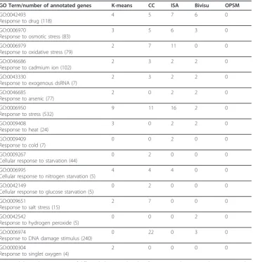
that is, to compare biclustering methods on the basis of which of them recover known patterns in the particular experimental dataset used. Table 3 shows the differences between the bicluster contents based on their predictability to recover the response to stress category. Although OPSM showed a high percentage of enriched biclusters, it had no biclusters with genes matching any of the known GO categories for the Gasch data set. Although there were few ISA biclusters (9) and a low percentage of gene cov-erage (25%), it showed better performance with one of its biclusters having 11 genes matching response to oxidative stress (GO:0006979). We also see that three methods (k-means, CC and ISA) were able to define biclusters with 4 out of 5 genes in the cel-lular response to nitrogen starvation functional category, which is very striking. Finally, we observe that several methods appear to be unique in detecting biclusters related to certain function categories. For example, ISA and CC detected two genes belonging to response to cold and cellular response to starvation functions, respectively.

The comparison methodology used in this study indicates that the present methods show no clear winner, and in fact it seems that all methods should somehow be inte-grated together to capture the information in the data (i.e. biclustering algorithms dif-fer in strategy, approach, time complexity, number of parameters and predictive Figure 2Percentage of enriched biclusters. The percentage of enriched biclusters for Biological Process GO annotations (y-axis) is shown against the selected biclustering algorithms (x-axis) at different

significance levels. Biclustering algorithms and k-means were applied to the Gasch dataset [19] using the parameter settings in Table 1 with GO annotations of the Biological Process category. A bicluster is said to be significantly overrepresented (enriched) with a functional category if the P-value of this functional category is lower than the preset threshold P-value. The OPSM algorithm gave a high portion of functionally enriched biclusters at all significance levels (from 85% to 100%). Next to OPSM, ISA shows relatively high portions of enriched biclusters.

capacity, so we expect that each algorithm can recover what other algorithms cannot. So on inspection of Table 3, we recommend biologists to run all biclustering algo-rithms on their data set and select the enriched results.)

As Friedman used the Spellman [20] cell cycle dataset, we applied BicAT-Plus to this dataset. We used the parameter settings shown in Table 4 and produced the biclusters shown in Table 5. One remarkable observation is that the gene coverage percentage of the ISA algorithm differs from the Spellman dataset (91%) (see Table 5) and the Gasch dataset (25%) (see Table 2). This confirms that each dataset has its unique signature, so integrating more than one dataset enables biological knowledge to be extracted that could not be extracted from a single dataset.

Table 3 Comparing biclustering algorithms on the basis of their predictive capacities for recovering selected patterns.

GO Term/number of annotated genes K-means CC ISA Bivisu OPSM

GO:0042493

Response to drug (118)

4 5 7 6 0

GO:0006970

Response to osmotic stress (83)

3 5 6 3 0

GO:0006979

Response to oxidative stress (79)

2 7 11 0 0

GO:0046686

Response to cadmium ion (102)

2 3 2 2 0

GO:0043330

Response to exogenous dsRNA (7)

2 3 2 2 0

GO:0046685

Response to arsenic (77)

2 0 2 2 0

GO:0006950

Response to stress (532)

9 11 16 2 0

GO:0009408 Response to heat (24)

3 0 2 2 0

GO:0009409 Response to cold (7)

0 0 2 0 0

GO:0009267

Cellular response to starvation (44)

0 2 0 0 0

GO:0006995

Cellular response to nitrogen starvation (5)

4 4 4 0 0

GO:0042149

Cellular response to glucose starvation (5)

0 2 0 0 0

GO:0009651

Response to salt stress (15)

2 7 0 0 0

GO:0042542

Response to hydrogen peroxide (5)

0 0 0 2 0

GO:0006974

Response to DNA damage stimulus (240)

0 22 0 3 0

GO:0000304

Response to singlet oxygen (4)

2 0 0 0 0

Network Validation

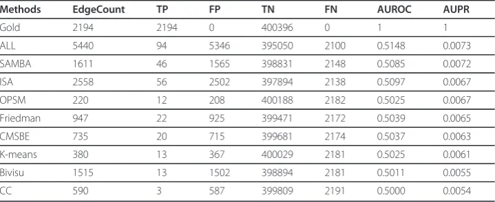
Figure 4 and Table 6 show the performance of the biclustering networks via the gold network retrieved by BioNetBuilder [33] and the Friedman network [4]. Inspecting Fig-ure 4 and Table 7, we find that neither the networks generated from different bicluster algorithms nor theALL networkperform well. There are two important considerations when interpreting the results of this comparison. First, the interactions documented are either physical or genetic. This implies that they may not be direct interactions. The precision may be lower than the actual precision since links may be missing in the interactome databases; and the recall may be lower than the actual recall in part because some of the links reported in the interactome databases may be indirect [39]. Second, some presently unsupported edges in the constructed network may find Table 4 Parameter settings of biclustering algorithms applied to the Spellman dataset [20].

Algorithm Parameters Parameter Description

ISA tg = 2.0 Gene threshold level tc = 2.0 Condition threshold level SN = 500 No of seeds

CC Delta = 0.5 Maximum accepted score Alpha = 1.2 Scaling factor

M = 100 Number of biclusters to be found

OPSM l = 100 Number of passed models for each iteration K-means M = 100 Number of biclusters to be found

IN = 100 Number of Iterations RN = 10 Number of replications

DM = ED Distance Metric is Euclidean Distance Bivisu NT = 0.5819 Data noise threshold

% NR = 1.57 Minimum% of rows

NC = 5 Minimum number of columns O% = 25% Maximum overlap allowed MSBE alpha = 0.4 Similarity threshold

beta = 0.5 Bonus similarity threshold

gamma = 1.2 Threshold of the average similarity score SAMBA MHS = 100 Maximal memory allocated for hashing

KHS1 = 4 stage

PC = 100 Maximal kernel size in the hashing stage

KHS2 = 4 Minimal number of responding probes per condition

O% = 25% Minimal kernel size in the hashing stage Maximum overlap between two biclusters

Parameter settings of biclustering algorithms applied to cell cycle gene expression data ofS. cerevisiaeprovided by Spellman et al. [20]. For more details about these parameters, see the corresponding publication.

Table 5 Statistical comparison of bicluster outputs using the Spellman dataset [20].

Biclustering Algorithm No of Biclusters GeneCoverage% ConditionCoverage%

Kmeans 100 100 100

ISA 219 91 100

CC 69 100 100

OPSM 12 84 57

BiVisu 100 62 100

experimental evidence in the future. Therefore, these unsupported edges are not neces-sarily false [40].

For the above reasons, the False Positive (FP) edges could be considered True Posi-tive (TP) if supporting evidence were found in the interaction databases (gold net-work). For example, if the inference network includes an edge between gene1 and gene3, which does not exist in the gold network, and if these two genes were con-nected indirectly via another intermediate gene such as gene2, we can now consider the edge between gene1 and gene3 to be a true positive edge. To be entirely consistent we change TN edge into a FN every time there is an interaction via an intermediate gene.

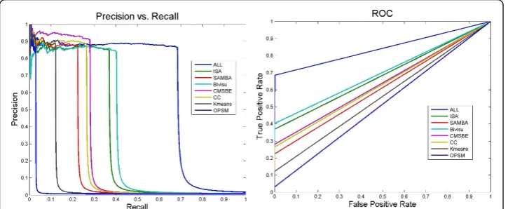
Table 8 and Figure 5 show the improvement in performance of the networks after taking the above evaluation modification into consideration. Furthermore, they show Figure 4ROC and PR curves of different biclustering networks that have learned using Bayesian networks[29]. A performance comparison of networks generated from learning corresponding

biclustering algorithms using the Bayesian networks method via the Friedman network [4] and the gold network retrieved by BioNetBuilder [33]. This figure shows that most of these networks contained few true positive edges. Neither the networks generated from different bicluster algorithms nor those generated from all biclustering networks (dashed line) perform well. ALL: This network is produced by integrating edges from all biclustering networks; Friedman Network [4]; SAMBA: This network is generated by integrating SAMBA [43] subnetworks; Kmeans: This network is generated by integrating k-means subnetworks; ISA: This network is generated by integrating ISA [31] subnetworks; OPSM: This network is generated by integrating OPSM [23] subnetworks; CC: This network is generated by integrating CC [24] subnetworks; Bivisu: This network is generated by integrating Bivisu [32] subnetworks; CMSBE: This network is generated by integrating MSBE [27] subnetworks.

Table 6 Number of network edges generated from different biclustering algorithms and Friedman network.

Bicluster Network Number of Edges

K-means network 380

ISA network 2558

OPSM network CC network 220 590

Bivisu network 1515

MSBE network 735

SAMBA network 1611

Total Number of Edges(ALL Network) 5440

Friedman Network 947

how most of the false positive edges in these networks have evidence in the gold net-work (the seventh column in Table 8).

It should be mentioned that, as we expected, the sparse nature of the GNR makes biclustering techniques (ISA, SAMBA, Bivisu) outperform the Friedman network. This promotes the use of biclustering algorithms to overcome the dimensionality problem in GRN inference.

As the success of biclustering algorithms in grouping functionally related genes (i.e. producing highly enriched biclusters), the corresponding learned subnetworks contain many true positive edges. This explains the performance difference in Table 8. So the challenge to produce a real network is reflected in finding enriched biclusters. Figures 2 and 3 and table 3 explain the high and low performance of algorithms ISA and OPSM, respectively. As ISA produces highly enriched biclusters (Figures 2 and 3) and is able to recover the selected pattern (Table 3), it produced a more realistic network; the opposite was the case for the OPSM algorithm. On the other hand, the ISA net-work even outperforms the SAMBA netnet-work: SAMBA produces fewer biclusters than ISA and recovers a lower percentage (see Table 5).

Table 7 Performance comparison of the biclustering networks.

Methods EdgeCount TP FP TN FN AUROC AUPR

Gold 2194 2194 0 400396 0 1 1

ALL 5440 94 5346 395050 2100 0.5148 0.0073

SAMBA 1611 46 1565 398831 2148 0.5085 0.0072

ISA 2558 56 2502 397894 2138 0.5097 0.0067

OPSM 220 12 208 400188 2182 0.5025 0.0067

Friedman 947 22 925 399471 2172 0.5039 0.0065

CMSBE 735 20 715 399681 2174 0.5037 0.0063

K-means 380 13 367 400029 2181 0.5025 0.0061

Bivisu 1515 13 1502 398894 2181 0.5011 0.0055

CC 590 3 587 399809 2191 0.5000 0.0054

Performances of biclustering networks are compared with the Friedman network and gold network. EdgeCount: the number of network edges; TP: number of true positive edges; TN: number of true negative edges; FP: number of false negative edges; AUROC: area under ROC curve; AUPR: area under precision recall curve.

Table 8 Performance comparison of the biclustering network using new evaluation criteria.

Methods EdgeC ount TP FP TN FN FP to TP TN to FN AURO C AUPR

Gold 2194 2194 0 400396 0 0 0 1 1

ALL 5440 94 5346 395050 2100 4623 2150 0.7530 0.4614

SAMBA 1611 46 1565 398831 2148 1340 2501 0.6958 0.3644

ISA 2558 56 2502 397894 2138 2141 1151 0.8451 0.6306

OPSM 220 12 208 400188 2182 190 2453 0.5423 0.089

Friedman 947 22 925 399471 2172 794 2700 0.6364 0.2491

CMSBE 735 20 715 399681 2174 653 2750 0.6181 0.2333

K-means 380 13 367 400029 2181 323 3100 0.5667 0.1307

Bivisu 1515 13 1502 398894 2181 1265 2610 0.6845 0.3326

CC 590 3 587 399809 2191 507 2800 0.5943 0.1788

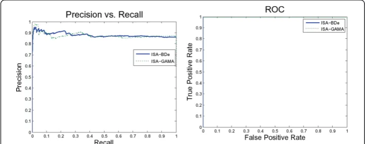
We also tried more than scoring functions. Figure 6 suggests that the ISA network performs equally using NormalGamma and the BDe scoring function. On the other hand, Figure 7 demonstrates that the ISA network using GreedyHillClimbing outper-formed the SparseCandidate algorithm with a different size of candidate sets. Further-more, decreasing or increasing the size of the candidate sets beyond five affects the network performance negatively.

To examine whether the performance on the datasets is typical of all network recon-struction methods and is not particular to Bayesian networks with biclustering, we ran another construction algorithm (linear regression) and compared the resultant net-works with those generated from the Bayesian netnet-works method. We used the LASSO algorithm, which is implemented in Faisal et al. [41] at the Helsinki Institute for Infor-mation Technology (http://users.ics.tkk.fi/faisal/Softwares/LassoRegression.tar.gz).

Figure 5ROC and PR curves of biclustering networks using modified evaluation methodology. The poor result of the previous figure (Figure 4) should be considered with regard to two important issues. First, some of the links reported in the interactome databases may be indirect rather than the direct. Second, the available interactome databases are still incomplete, so the false positive edges that are unsupported are not necessarily false and may find experimental evidence in the future. The False Positive (FP) edges could be considered True Positive (TP) if they have evidence in the literature (gold network). For example, if the inference network includes an edge between gene1 and gene3, which does not exist in the gold network, and if these two genes connect indirectly via another intermediate gene such as gene2, we can now consider the edge between gene1 and gene3 as a true positive edge. To be entirely consistent we change a TN edge into FN every time there is an interaction via an intermediate gene.

We used the cross-validation method to determine the best optimum lambda. Figure 8 shows network performances using linear regression. Comparing Figure 8 with the Bayesian results in Figure 5, we find the following:

•The performance of the CMSBE network does not change significantly.

•The performances of the ALL, OPSM and Bivisu, networks are greater using the LASSO method than with the Bayesian networks method.

•The performances of the ISA, SAMBA and K-means, networks are lower using the LASSO method than with the Bayesian networks method.

Figure 7ISA network performance using different search algorithms. Network performance using Greedy Hill Climbing outperformed the SparseCandidate learning algorithm. For the SparseCandidate algorithm, decreasing or increasing the size of the candidate sets beyond five worsens the network performance.

We could conclude from Figures 5 and 8 that while different network reconstruction algorithms will lead to differences in absolute performance, different biclustering schemes consistently have similar relative performances, irrespective of the network reconstruction algorithm used.

Furthermore, analyzing network topology increases the credibility of the predicted network. We therefore analyzed the ISA network and the gold network using NET-WORKANALYZER [36]. Table 9 shows that these three important parameters are the same in the two networks, indicating the high performance of the ISA network.

Finally, one of the best methods for validating a network is to assess its accumulated information using the information published in the biological literature. Clustering algorithms have been used to identify molecular complexes or modules in a large pro-tein interaction network through network connectivity [37]. A network module is a group of nodes in the network that work together to execute some common function. We used the MCODE Cytoscape plug-in [37] to detect densely connected regions in the ISA network, which retrieved 39 modules. Figure 9 shows the highly scored mod-ules with the number of nodes and edges and the topology of each module discovered. To validate the significance of the recovered modules, their nodes are a portion of a complex, so there should be some process in which they all operate. Thus, if we explore Gene Ontology (GO) term enrichment using functional enrichment tools such as BINGO [38], we should see some biological process with significant enrichment for these nodes [42]. Figure 10 demonstrates the functional enrichment of a highly scored module using BINGO [38], which indicated that the module genes share three related biological process: Chromatin assembly or disassembly, DNA Packaging and Establish-ment and/or Maintenance of Chromatin Architecture.

Conclusions

The ongoing development of high-throughput technologies such as microarray prompts researchers to study the complexity of gene regulatory networks (GRNs) in cells. GRN inference algorithms have significant impact on drug development and on understanding of disease ontology. Many GRN inference algorithms based on genome-wide data have been developed to unravel the complexity of gene regulation. Tran-scriptomic data measured by genome-wide DNA microarrays are traditionally used for GRN modelling. This is because RNA molecules are more easily accessible than pro-teins and metabolites. One of the major problems with time series microarrays is that a dataset consists of relatively few time points with respect to a large number of genes. Reducing the data dimensions is one of the interesting problems in GRN modelling. The most common and important design rule for modelling gene networks is that their topology should be sparse. This means that each gene is regulated by only a few

Table 9 Analyzing the topologies of the ISA and gold networks using NetworkAnalyzer [36].

Parameters Gold Standard Network ISA Network

Network Diameter 8 9

Network Density 0.011 0.012

Avg. no of neighbors 6.91 6.933

biclustering algorithms in GRN construction. Sophisticated filtration procedures such as data filtration, missing value imputation, normalization and discretization were used to reduce the number of expression profiles to some subset that contains the most sig-nificant genes.

Also, the biclustering comparison toolbox (BicAT-Plus) implemented in this paper confirms that the bicluster and cluster algorithms can be considered as an integrated module; there is no single algorithm that can recover all the interesting patterns. What algorithm A recovers in certain data sets, Algorithm B might fail to recover, and vice versa. We can identify the highly enriched biclusters in all the algorithms compared, integrating them to solve the dimensionality problem of GRN construction.

Moreover, the study in this paper confirms the ability of Bayesian Networks (BNs) structure algorithms to recover gene network structures accurately. BNs allow us to deal with the noise inherent in experimental measurements and to model the hidden variables in the data.

MCODE and NetworkAnalyzer adds more credibility to our algorithm. The data used in the validation step is not used for modelling. On the other hand, putative modules were recovered from our method, which suggests the need for more analysis to recover and test unknown complex modules.

We implemented the algorithm in Java. The program is open source and can be obtained from the authors.

Acknowledgements

This work is supported by a grant from the University of Science & Technology, Yemen. The authors would like to thank Prof Dana Pe_’er, Columbia University; Dr Kevien Yip, Yale University and Prof G. Stolovitzky, IBM Computational Biology Center for helpful discussions. We also thank Stanford Microarray Database for making microarray data available and the lab members for the courteous help they gave us.

Author details

1

University of Science and Technology, Sana’a, Yemen.2Department of Biomedical photonics, Niles, Giza, (12613), Egypt.3_{Department of Biomedical Engineering, Cairo University, Giza, (12613), Egypt.}

Authors’contributions

The initial idea of the algorithm was developed by all the authors. FA developed and tested the software. All the authors wrote and approved the manuscript.

Competing interests

The authors declare that they have no competing interests.

Received: 9 May 2011 Accepted: 22 October 2011 Published: 22 October 2011

References

1. Ronald CT, Mudita S, Jennifer W, Saeed K, Liang S, Jason M:A Network Inference Workflow Applied to Virulence-Related Processes in Salmonella typhimurium.Ann N Y Acad Sci2009,1158:143-158.

2. Dyer MD, Murali TM, Sobral BW:The Landscape of Human Proteins Interacting with Viruses and Other Pathogens.

PLoS Pathog2008,4:e32.

3. Kauffman S:Homeostasis and Differentiation in Random Genetic Control Networks.Nature1969,224(5215):177-178. 4. Friedman N, Linial M, Nachman I, Pe’er D:Using Bayesian networks to analyze expression data.Proceedings of the

fourth annual international conference on Computational molecular biology; Tokyo, JapanACM; 2000, 127-135, 332355. 5. Wolfe C, Kohane I, Butte A:Systematic survey reveals general applicability of“guilt-by-association’’within gene

coexpression networks.BMC Bioinformatics2005,6(1):227.

6. D haeseleer P, Wen X, Fuhrman S, Somogyi R:Linear modeling of mRNA expression levels during CNS development and injury.4th Pacific Symposium on BiocomputingBig Island of Hawaii; 1999.

7. Chen T, Hongyu LH, Church GM:Modeling gene expression with differential equations.4th Pacific Symposium on BiocomputingBig Island of Hawaii; 1999.

8. Tavazoie S, Hughes J, Campbell M, Cho R, Church G:Systematic determination of genetic network architecture.

Nature Genetics1999,22:281-285.

9. Guthke R, Moller U, Hoffmann M, Thies F, Topfer S:Dynamic network reconstruction from gene expression data applied to immune response during bacterial infection.Bioinformatics2005,21(8):1626-1634.

10. D’haeseleer P, Liang S, Somogyi R:Genetic network inference: from co-expression clustering to reverse engineering.

Bioinformatics2000,16(8):707-726.

11. Reiss D, Baliga N, Bonneau R:Integrated biclustering of heterogeneous genome-wide datasets for the inference of global regulatory networks.BMC Bioinformatics2006,7(1):280.

12. Prelic A, Bleuler S, Zimmermann P, Wille A, Buhlmann P, Gruissem W, Hennig L, Thiele L, Zitzler E:A Systematic comparison and evaluation of biclustering methods for gene expression data.Bioinformatics2006,22(9):1122-1129. 13. Madeira SC, Oliveira AL:Biclustering algorithms for biological data analysis: a survey.IEEE/ACM Trans Comput Biol

Bioinform2004,1(1):24-45.

14. Yeung KY, Haynor DR, Ruzzo WL:Validating clustering for gene expression data.Bioinformatics17(4):309-318. 15. Datta S, Datta S:Comparisons and validation of statistical clustering techniques for microarray gene expression

data.Bioinformatics2003,19(4):459-466.

16. Azuaje F:A cluster validity framework for genome expression data.Bioinformatics2002,18(2):319-320. 17. Barkow S, Bleuler S, Prelic A, Zimmermann P, Zitzler E:BicAT: a biclustering analysis toolbox.Bioinformatics2006,

22(10):1282-1283.

18. Bonneau R, Reiss D, Shannon P, Facciotti M, Hood L, Baliga N, Thorsson V:The Inferelator: an algorithm for learning parsimonious regulatory networks from systems-biology data sets de novo.Genome Biology2006,7(5):R36. 19. Gasch AP, Spellman PT, Kao CM, Carmel-Harel O, Eisen MB, Storz G, Botstein D, Brown PO:Genomic Expression

Programs in the Response of Yeast Cells to Environmental Changes.Mol Biol Cell2000,11(12):4241-4257. 20. Spellman PTSG, Zhang MQ, Iyer VR, Anders K, Eisen MB, Brown PO, Botstein D, Futcher B:Comprehensive

identification of cell cycle-regulated genes of the yeast Saccharomyces cerevisiae by microarray hybridization.Mol Biol Cell1998,9(12):3273-3297.

22. Isaac SK, Alvin K, Atul JB:Microarrays for an Integrative Genomics..

23. Ben-Dor A, Chor B, Karp R, Yakhini Z:Discovering local structure in gene expression data: the order-preserving submatrix problem.Journal of Computational Biology2003,10:373-384.

24. Cheng Y, Church GM:Biclustering of expression data.Proceedings of 8th International Conference on Intelligent Systems for Molecular Biology2000, 93-103.

25. Murali TM, S K:Extracting conserved gene expression motifs from gene expression data.Pac Symp Biocomput2003, 77-88.

26. Fung G:A Comprehensive Overview of Basic Clustering Algorithms.Citeseer2001, 1-37.

27. Liu X, Wang L:Computing the maximum similarity bi-clusters of gene expression data.Bioinformatics2007, 23(1):50-56.

28. Al-Akwaa FM, Kadah YM:Comparison Performance of Structure Learning Bayesian Network Algorithms Based on Gene Expression Data.4th Cairo International Biomedical Engineering Conference; Cairo, Egypt2008.

29. Dana Pe:Bayesian Network Analysis of Signaling Networks: A Primer.Sci STKE2005,2005(281):l4.

30. Alakwaa FM:A novel microarray denosing algorithm using spectral subtraction.Biomedical Engineering (MECBME) 2011 1st Middle East Conference on; Sharjah2011, 167-169.

31. Ihmels J, Friedlander G, Bergmann S, Sarig O, Ziv Y, Barkai N:Revealing modular organization in the yeast transcriptional network.Nature Genetics2002,31:370-377.

32. Cheng KO, Law NF, Siu WC, Lau TH:BiVisu: software tool for bicluster detection and visualization.Bioinformatics

2007,23(17):2342-2344.

33. Avila-Campillo I, Drew K, Lin J, Reiss DJ, Bonneau R:BioNetBuilder: automatic integration of biological networks.

Bioinformatics2007,23(3):392-393.

34. Stolovitzky G, Prill R, Califano A:Lessons from the DREAM2 Challenges.Annals of the New York Academy of Sciences

2009,1158:1159-1195.

35. Jesse D, Madison W:The relationship between Precision-Recall and ROC curves.Proceedings of the 23rd international conference on Machine learningACM New York, NY, USA; 2006, 233-240.

36. Assenov Y, Ramirez F, Schelhorn SE, Lengauer T, Albrecht M:Computing topological parameters of biological networks.Bioinformatics2008,24(2):282-284.

37. Bader G, Hogue C:An automated method for finding molecular complexes in large protein interaction networks.

BMC Bioinformatics2003,4(1):2.

38. Maere S, Heymans K, Kuiper M:BiNGO: a Cytoscape plugin to assess overrepresentation of Gene Ontology categories in Biological Networks.Bioinformatics2005,21(16):3448-3449.

39. Lozano AC, Abe N, Liu Y, Rosset S:Grouped graphical Granger modeling for gene expression regulatory networks discovery.Bioinformatics2009,25(12):i110-118.

40. Chen Xw, Anantha G, Wang X:An effective structure learning method for constructing gene networks.

Bioinformatics2006,22(11):1367-1374.

41. Faisal A, Dondelinger F, Husmeier D, Beale CM:Inferring species interaction networks from species abundance data: A comparative evaluation of various statistical and machine learning methods.Ecological Informatics2010, 5(6):451-464.

42. Shannon P, Markiel A, Ozier O, Baliga N, Wang J, Ramage D, Amin N, Schwikowski B, Ideker T:Cytoscape: a software environment for integrated models of biomolecular interaction networks.Genome Res2003,13(11):2498-2504. 43. Tanay A, Sharan R, Shamir R:Discovering statistically significant biclusters in gene expression data.Bioinformatics

2002,18(suppl_1):S136-144.

doi:10.1186/1742-4682-8-39

Cite this article as:Alakwaaet al.:Construction of Gene Regulatory Networks using biclustering and Bayesian

networks.Theoretical Biology and Medical Modelling20118:39.

Submit your next manuscript to BioMed Central and take full advantage of:

• Convenient online submission

• Thorough peer review

• No space constraints or color figure charges

• Immediate publication on acceptance

• Inclusion in PubMed, CAS, Scopus and Google Scholar

• Research which is freely available for redistribution