Solving Two-Points Singular Boundary Value Problem Using Hermite Interpolation Heba A. Abd Al-Razak

(1)

Baghdad Science Journal

Vol.12(4)2015

Solving Two-Points Singular Boundary Value Problem

Using Hermite Interpolation

Heba A. Abd Al-Razak

Department of Mathematics, College of Science for Women, University of Baghdad.

Received 3, September, 2014 Accepted 5, February, 2015

This work is licensed under a Creative Commons Attribution-NonCommercial-NoDerivatives 4.0 International Licens

Abstract:

In this paper, we have been used the Hermite interpolation method to solve second order regular boundary value problems for singular ordinary differential equations. The suggest method applied after divided the domain into many subdomains then used Hermite interpolation on each subdomain, the solution of the equation is equal to summation of the solution in each subdomain. Finally, we gave many examples to illustrate the suggested method and its efficiency.

Keywords

:

Singular ordinary differential equations, Boundary value problems, Hermite interpolation.

Introduction:

Singular boundary value problems (SBVP's) for ordinary differential equations (ODE) arise very frequently in several areas of science and engineering. For example, in analysis of heat conduction through a solid with heat generation, Thomas–Fermi model in atomic physics, electro hydrodynamics and the theory of thermal explosions. These arise in Physiology as well in the study of various tumor growth problems, in the study of the distribution of heat sources in the human head[1-3]. Singular boundary value problems are always very important, there exists many method for solving. For example, modified Homotopy perturbation method [4], differential transform method [5],

cubic trigonometric B-spline

method[6], Adomian decomposition method [7], shooting method [8], variation method[9].

Hermite interpolation method which was mooted by charts Hermite is often used in interpolation of the data points when the derivative of the function f(x) in the given points are available this technique has superiority on the other types of interpolation polynomial [10]. In this paper we will use Hermite

interpolation method for solving

singular boundary value problems of ODE after divided the interval [0,1] into many subdomains equal distance. Numerical examples show that present method is efficiency.

1. Hermite Interpolation [11]

(2)

polynomial, i.e., the interpolation problem can also be formulated in another way, viz. as the answer to the following question : How to find a good representative of a function that is not knew explicitly, but only at some points of the domain of interest. In this paper we will consider Hermite interpolation where the interpolation polynomial also matches the first

derivatives ( )( ) . This

interpolation technique is important since it has the property that gives high order of accuracy.

Theorem 1:[11] Suppose that f(x)

[a,b] , and that

are distinct, then the unique polynomial of degree (at most) 2n + 1

denoted by , and such that :

( ) ( ) ( )

( ) is given by : ( ) ∑ [ ( )(

)] ( ) ( ) ∑(

) ( ) ( ) …(1)

( ) ∏

The error bound for Hermite interpolation is provided by the expression:

E=( ) ( ) (

) ( )_{( ) ( )}_,where

f(x) .

2. Singular Boundary Value Problem

The general form of the order

two point boundary value problems (TPBVP) is:

_{( )} _{( )}

( )

With the boundary conditions

(BC):y(a) = A and y(b) = B, where A, B ϵ R

There are two types of a point [0,1].Ordinary point and Singular

point.A function y(x) is analytic at if

it has a power series expansion at that converges to y(x) on an open

interval containing . A point is an

ordinary point of the ODE (2), if the functions P(x)and Q(x) are analytic at

. Otherwise is a singular point of

the ODE. On the other hand if P(x)

or Q(x) are not analytic at then is

said to be a singular point [12-13].There is at present, numerical method for solving problems with regular singular points using Hermite interpolation method with interval [0 1].

3. Description of the Method

In this section ,we apply the Hermite

interpolation method and Taylor

series to solve regular differential

equations. A general form of the

order SBVP's is:

₍₎

( )

Subject to the boundary condition (BC):

In the case Dirichlet BC: y(0)= A, y(1) = B, where A, B ϵ R

In the case Neumann BC: y′(0)= A, y′(1) = B, where A, B ϵ R

In the case Cauchy or mixed BC: y(0)= A, y′(1) = B, where A, B ϵ R

Or y′(0)= A, y(1) = B, where A, B ϵ R

where f is a general nonlinear function . Now, to solve the problem by the suggested method we will doing the following steps:

Step one: Evaluate Taylor series of y(x) about x = 0:

( ) ∑

∑ ( )

Where y(0)= ,y'(0)= ,

_{( )}

= ,…,

( )_{( )}

,i=3,4,…

Evaluate Taylor series of y(x) about x = 1/3:

( ) ∑ ( ) ( ) ∑ ( ) ( )

Where y(1/3)= ,y'(1/3)= , ( )

= ,…,

( )_{( )}

(3)

Evaluate Taylor series of y(x) about x = 2/3:

( ) ∑ ( ) ( ) ∑ ( ) ( )

Where y(2/3)= ,y'(2/3)= ,

_{( )}

= ,…,

( )_{( )}

,i=3,4,…

And evaluate Taylor series of y(x) about x = 1:

( ) ∑ ( )

( ) ∑ ( ) ( )

Where y(1)= ,y'(1)= , ( )

= ,…,

( )_{( )}

,i=3,4,…

Step two: Insert the series form (4) with derivatives into equation (3) and put x = 0, then equate the coefficients of powers of x to obtain

.Then derive equation(3) with respect to x,to get new form of equation say(8) as following:

_{( )} _{( )} ( )

( )

Then insert the series form (4) with derivatives into equation (8) and put x=0 equate the coefficients of power of

x to obtain .Iterate this process

many times to obtain then and so

on.

Step three: Make up x=1/3 into

equation (4) to obtain y(1/3)= ,to

find derive the equation(4)and

requite x=1/3,and insert the series (5) into equation (3) and put x=1/3,then equate the coefficients of power of

(x-1/3) to obtain .to find insert the

series (5) into equation (8) and put x=1/3 and equate the coefficient of power of (x-1/3). Iterate this process

on.

Step four: Make up x=2/3 into

equation (5) to obtain y(2/3)= ,to

find derive the equation(5)and

requite x=2/3,and insert the series (6) into equation (3) and put x=2/3,then equate the coefficients of power of

(x-2/3) to obtain .to find insert the

series (6) into equation (8) and put x=2/3 and equate the coefficient of power of (x-2/3). Iterate this process

on.

Step five: Insert the series form (7) with derivatives into equation (3) and put x = 1, then equate the coefficients of powers of( x-1) to

obtain ,to find insert the

series(7) with derivatives into equation (8) and put x=1 and equate the coefficient of power of (x-1) . Iterate this process many times to obtain

then and so on.

Step six: The notation implies that the coefficients depend only on the

indicated unknowns

where dependes on the

indicated unknowns

When the substitute (BC) we get two

unknown coefficients and then

substitute for coefficients ( )

that we have obtained the previous

steps in Hermite interpolation

polynomial equation(1).

Step seven: To find the unknown

coefficients by reduction order

equation and use as a

replacement of y(x) and substitute the boundary conditions , we have only

two unknown coefficients from

and two equation, we can find this for any n by solving this system of algebraic equations. So insert the value of the unknown coefficients into equation (1),Thus equation (1) represent the solution of the problem.

4. Error Estimation for SBVP's

(4)

an estimate of the error or maximum defect is being used. If the error is being uses estimated, in this paper we modify this package to consist SBVPs, defined as :

E= (x)- (x) / ( 1 +

(x) ) ; 0

where y(x) is exact solution and

(x) is suggested solution of SBVPs . If the exact solution does not find then the component error of SBVPs is

E= ''(x) − f(x, (x),

'(x)) / ( 1 + f(x, (x), '(x) ) )

The relative estimate of both the error and the maximum defect are slightly modified from the one used in SBVP SOLVER[ 14] .

5. Numerical Examples:

In this section ,we used Hermite interpolation and Taylar series to solve singular boundary value problems (SPVBs).After the domain [0 ,1] is divided into two points with points 0,1

where you found polynomial

solution (x) and presented the

results the Variational iteration method and the exact solution, and the domain [0 ,1] is divided into four points with points 0,1 where you found

polynomial solution (x),also the

domain[0 ,1] is divided into night points with points 0,1 where you found

polynomial solution (x).Then

examples calculated maximum error in each case n=4,6,11 with figure polynomials to find a good solution.

Example1. Consider the following SBVP :

( )

, 0 ≤ x ≤ 1

with mixed BC:y'(0) = 0, y(1) = 1.

The exact solution is : y(x) =1- [15]

Using Taylor polynomials ,we have y(0)=1 ,y(1/3)= 0.8888888888888889, y(2/3)= , 0.5555555555555555

y'(1/3)= -0.6666666666666667,

y'(2/3)= 1.333333333333333, y'(1)= -2

Now, we solve this equation using these data

( )= 9.148237723 -

3.268496584 +

4.227729278 -

2.664535259 +

7.860379014 - 1.0 + 1.0

Geng [15] solved this example by (VIM) and give the following series solution:

p (x) = 0.999997 - + 1.2347

₊ _1.46988 ₊

0.0000165329

-0.0000201421 +7.95888

-1.03072

The numerical results are given in

following Table 1 gives ( ) and

result VIM also exact solution. Table 2 gives the maximum error for number point n = 4 , 6, 11. Figure 1 gave the accuracy of the suggested method.

Table 1: Numerical results for n=4 of example 1

VIM p(x) Hermite

interpolation

( )

Exact Solution y(x) xi

0.999997000000000 1

1

0

0.989997000012525 0.990000000000000

0.990000000000000

0.1

0.959997000238787 0.960000000000000

0.960000000000000

0.2

0.909997001980789 0.910000000000001

0.910000000000000

0.3

0.839997012074748 0.840000000000001

0.840000000000000

0.4

0.749997054738341 0.750000000000002

0.750000000000000

0.5

0.639997189102191 0.640000000000003

0.640000000000000

0.6

0.509997518669322 0.510000000000004

0.510000000000000

0.7

0.359998167043863 0.360000000000005

0.360000000000000

0.8

0.189999194602654 0.190000000000007

0.190000000000000

0.9

4.57128800035456e-07

8.43769498715119e-15 0

1

Table 2: The result maximum error when n=4,6,11of example 1

Hermite interpolatio

n ( )

n ( ) Er

ror

3.03624319 630824e-07 2.31020758

079126e-12 4.21884749

357560e-15 M.

(5)

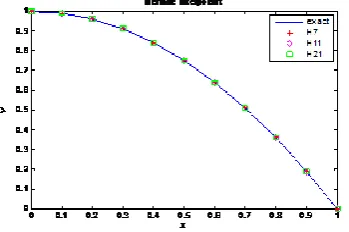
Fig.1: Comparison between the exact and suggested solution when n= 4, 6,11

Example2

. Consider the following

SBVP : ,

0 ≤ x ≤ 1

with mixed BC:y'(0) = 0, y(1) = 5.5.

The exact solution is : y(x) =

( ) ( ) [15]

Using Taylor polynomials, we have y(0)= 3.257205700320381 ,y(1/3)=

3.466030095098947, y(2/3)=

4.1499242047031

y'(1/3)= 1.280759726616932, y'(2/3)=

2.915149400050196, y'(1)=

5.373147016441

( )= 0.009130738291121613 +

0.01920841575611729 +

0.01361484275073988 +

0.3613904331003707 +

0.001445668149072448 +

1.838004201632197 +

3.257205700320381

Geng [15] solved this example by (VIM) and give the following series solution:

p (x) = 3.25721 + 1.83814 +

0.367628 +

0.0350121 +0.00194512 +

0.0000707316

The numerical results are given in and

Table 3 gives ( ), results VIM exact

solution. Table 4 gives the maximum error for number point n = 4, 6, 11. Figure 2 gives the accuracy of the suggested method.

VIM p(x) Hermite

interpolation

( )

Exact Solution y(x) xi

3.27562819783156 3.27562348331808

3.27562381647618

0.1

3.33132605056115 3.33132136138556

3.33132158129189

0.2

3.42564603865789 3.42564145791085

3.42564142056487

0.3

3.56086836853219 3.56086354389276

3.56086353732463

0.4

3.74027648126133 3.74027129054089

3.74027136831943

0.5

3.96825161157128 3.96824615761122

3.96824614512855

0.6

4.25039935164274 4.25039351936955

4.25039346768551

0.7

4.59371217247398 4.59370563007463

4.59370586068823

0.8

5.00677296919957 5.00676603087337

5.00676642428200

0.9

5.50000595160000 5.50000000000000

5.50000000000000

1

Table 4: The result maximum error when n=4,6,11of example 2

Hermite interpolation

( ) Hermite

interpolation ( ) Hermite

interpolation

( )

Erro r

1.9597881395255 3e-05 3.2687191368661

6e-06 6.0524403950195

8e-08 M.E

Fig.2: Comparison between the exact and suggested solution when n=4,6,11

Example 3

. consider the following

SBVP: (1- x2) y"+ x y'+ y = 0 , 0

≤ x ≤ 1

With Neumann BC : y'(0) = 0, y'(1) = - y(1) [11]

Using Taylor polynomials, we have

y(0)= 1.85779174711865 ,y(1/3)=

2.076407841859629, y(2/3)=

2.02488427571492,y(1)=

1.65096790760441614054343517637,

y'(1/3)= 0.2793960039864789,

y'(2/3)= 0.6144298559221, y'(1)= -1.650967907604

7(x) -

0.001499602844631908737937919795

(6)

0.027426733964148297673091292381

287x5+ 0.07514319897959248x4-

0.332863322735647670924663543701

17x3 -

0.928936107025947421789169311523

44x2 + x + 1.857791747118655

The numerical results are given in

and Table 5 gives ( ), results VIM

exact solution. Table 6gives the maximum error for number point n = 4, 6, 11. Figure 3 gives the accuracy of the suggested method.

Hermite interpolation ( ) P7

xi

1.85779174711866 1.857784296228232

0

1.94817677138695 1.948169418187120

0.1

2.01808339018278 2.018075735440336

0.2

2.06574825787000 2.065740050052486

0.3

2.08953495227793 2.089526555233489

0.4

2.08791430899834 2.087906467474147

0.5

2.05944879456718 2.059442143114885

0.6

2.00278016273118 2.002774819034724

0.7

1.91661963799949 1.916615117147540

0.8

1.79973987068057 1.799735452392664

0.9

1.65096790760442 1.650963483906875

1

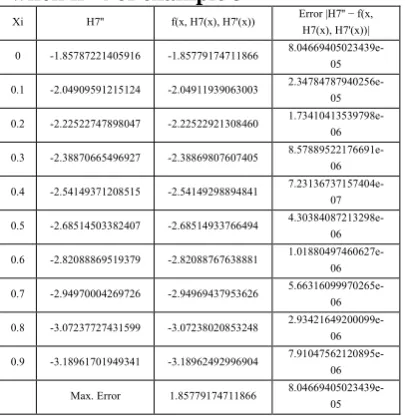
Table 6:the results maximum error when n=4 of example 3

Error |H7'' − f(x, H7(x), H7'(x))| f(x, H7(x), H7'(x))

H7'' Xi

8.04669405023439e-05 -1.85779174711866

-1.85787221405916 0

2.34784787940256e-05 -2.04911939063003

-2.04909591215124 0.1

1.73410413539798e-06 -2.22522921308460

-2.22522747898047 0.2

8.57889522176691e-06 -2.38869807607405

-2.38870665496927 0.3

7.23136737157404e-07 -2.54149298894841

-2.54149371208515 0.4

4.30384087213298e-06 -2.68514933766494

-2.68514503382407 0.5

1.01880497460627e-06 -2.82088767638881

-2.82088869519379 0.6

5.66316099970265e-06 -2.94969437953626

-2.94970004269726 0.7

2.93421649200099e-06 -3.07238020853248

-3.07237727431599 0.8

7.91047562120895e-06 -3.18962492996904

-3.18961701949341 0.9

8.04669405023439e-05 1.85779174711866

Max. Error

Where n=4,6,10, then max. error:

‖ _{( ) (} _{( )} _{( ))‖} ₍

‖ ( ( ) ( ))‖

‖ ( ) ( ( ) ( ))‖

( ‖ ( ( ) ( ) )‖

‖ ( ) ( ( ) ( ))‖ ( ‖ ( ( ) ( ) )‖ =

0.003949

Fig. 3: Comparison the suggested solution when n=4,6,11

Conclusion:

In this paper Hermite interpolation method was used to solving singular boundary value problem. The result shown that the divided the domain into a number point follow the same steps as the previous is a very powerful and efficient in finding accurate solution for a large class of regular singular point.

References:

[1] Kadalbajoo, M. K. and Kumar V. 2007. B-spline method for a class of singular two-point boundary value problems using optimal grid. Appl. Math. Computa., 188(2) : 1856-1869.

[2] Jamet, P., 1970.On the convergence of finite difference approximations

to one dimensional singular

boundary value problems. Numer. Math.,14(4): 355–378

(7)

[4] Mahmoudi, M. and Kazemi, M. V. 2013. Solving singular boundary

value problems of ordinary

differenal equation by modified homotopy perturbation method. Appl Math. Comput. Sci., (7):138-143.

[5] Ravi Kanth, A. S. V. and Aruna, K.

2008. Solution of singular two

point boundary value problems using differential transformation

method. Phys. Lett. A, 372(26):

4671–4673.

[6] Gupta, Y. and kumar, M. 2011. A Computer based numerical method

for singular boundary value

problems. Int. J. Comput. Applic. 30(1):21-25.

[7] Ebaid, A. and Aljouf, M. D. 2012. Exact solutions for a class of singular two-point boundary value

problems using adomian

decomposition Method. Appl.

Math. Sci.,6(122):

6108

-

6097

[8] Koch, O. and Weinmüller, E. B. 2003.The convergence of shooting methods for singular boundary value problems. math. Comput., 72(241): 289–305.

[9] Tripathi, B. k. 2013. Solution of a class of singular two point boundary value problems by

variational method. Math.

comput. Sci. res.,6(3):35-39.

[10] Butcher, J. C.; Corless, R. M.,

Gonzale, L. and shakoori-Vega, A. 2011. Polynomial algebra for

Birkhoff interpolants. Numer.

Algorith., 56(3) : 319-347.

[11] Burden, L. R. and Faires, J. D. 2001. Numerical analysis. Seventh Edition.

[12] Rachůnková, I.; Staněk, S. and Tvrdý, M. 2008. Solvability of Nonlinear Singular Problems for Ordinary Differential Equations. Hindawi, New York, pp279. [13] Shampine, F.; Kierzenka, J. and

Reichelt, M. W. 2000. Solving Boundary Value Problems for Ordinary Differential Equations in Matlab with bvp4c. The Math Works, Inc., 24 Prime Park Way, Natick,MA.,pp1-27.

[14] Carnahan, B.; Luther, H. and

Wilkes, J. 1990. Applied

numerical methods. Robert E.

Krieger Publishing Company,

Inc.,Florida , pp 604.

[15] Geng, F. 2010. Variational iteration method for a class of singular boundary value problems. Math. Sci., 4(4): 359-370.

جهريه جارذنلاا ماذختساب نيتطقنلا ثار ةراشلا تيدوذحلا نيقلا تلأسه لح

قازرلا ذبع داوع تبه

ثاٍضاٌشلا نسق ,ثانبلل مىلعلا تٍلك ,

داذغب تعهاج

:تصلاخلا

تٍناثلا تبحشلا نه تٍهاظنلا تٌدوذحلا نٍقلا لئاسه لحل جهشٍه جاسذنا تقٌشط انهاذخخسا,ثحبلا ازه ًف

. ةراشلا تٌداٍخعلاا تٍلضافخلا ثلاداعولل ذعب اهقٍبطح تقٌشط حشخقا

جولا نه ذٌذعلا ىلا لاجولا نٍسقح ا

لا تٍعشفلا ث

عشف لاجه لك ىلع جهشٍه جاسذنلاا ماذخخسا نث نهو . ً

.ًعشف لاجه لك ًف لحلا عوج يواسٌ تلداعولل لحلا

.هحءافكو حشخقولا بىلسلاا خضىخل تلثهلاا نه ذٌذعلا انهذق,اشٍخا

:تيحاتفولا ثاولكلا