ORIGINAL ARTICLE
T. Kawasaki (*) · K. Hwang · K. Komatsu · S. Kawai
Wood Research Institute, Kyoto University, Gokasho, Uji, Kyoto 611-0011, Japan
Tel. ⫹81-774-38-3677; Fax ⫹81-774-38-3678 e-mail: [email protected]
Part of this report was presented at the 50th Annual Meeting of the Japan Wood Research Society, Kyoto, Japan, April 2000; and the 5th Pacific Rim Bio-Based Composite Symposium, Canberra, Australia, December 2000
Tamami Kawasaki · Kweonhwan Hwang · Kohei Komatsu Shuichi Kawai
In-plane shear properties of the wood-based sandwich panel as a small
shear wall evaluated by the shear test method using tie-rods
dwelling houses. Low-density fiberboard has adequate ther-mal insulation properties to substitute for conventional in-sulation materials,3
and when sandwiched with veneers it was found to be viable for structural use.4
A wood-based sandwich panel of plywood-overlaid low-density fiberboard was manufactured in this study and in-plane shear properties were investigated to develop it as a shear wall. The shear test method for building construction5
was modified and applied to the sandwich panel as 260 mm square, regarding it a small shear wall. The test was also applied to plywood and low-density fiberboard.
The behavior of the sandwich panel was analyzed based on some originally proposed models, and its appropriate-ness was examined. Shear strength was also determined.
Experimental
Test specimen
Sandwich panels of plywood-overlaid low-density fiber-board (SW) were manufactured. For the core of the SW, fiber from lauan (Shorea spp.) was used that had been com-mercially produced using pressurized double disk refiner (PDDR) (Hokushin Co.). The resin adhesive was com-mercial polymeric methylene diphenyl diisocyanate (MDI) (Mitsui Takeda Chemical Co.). The resin content was 10% solid resin of MDI based on its oven-dried fiber weight.
Plywood was used for the face material of SW. It was commercially produced from weather- and boil-proof ply-wood (type special)6
of 9 mm thickness. It consisted of three plies of 3-mm layers of Japanese larch (Larix gmelini Gordon), with an average density of 0.68 g/cm3
. Before pressing, the MDI (UL-4811, Gun-ei Kagaku Kogyo Co.) was spread for internal bonding between the core and the face of the SW at 75 g/m2
(solid basis) for a bonding layer. The assembled fiber mat with faces was pressed once using the steam-injection pressing machine, heating from both sides.7
The target density range for SW was 0.35–0.40 g/ cm3
. The target thickness of SW was 100 mm, and the aver-Received: May 9, 2001 / Accepted: June 26, 2002
Abstract The fundamental in-plane shear properties were investigated for the wood-based sandwich panel of plywood-overlaid low-density fiberboard (SW) manufac-tured at a pilot scale to develop it as a shear wall. The shear test method using tie-rods standardized for shear walls was applied to SW with dimensions of 260 mm square and 96 mm thick as a small shear wall and to plywood (PW) and thick low-density fiberboard (FB). The shear modulus and shear strength of PW, FB, and SW were determined. To measure the shear deformation angle, a displacement meter and strain-gauge were used. The shear moduli of PW (0.68 g/cm3
) and FB (0.25–0.35 g/cm3
) were 460 and 21– 58 MPa/rad, respectively. The shear modulus of SW as a composite was analyzed. Some experimental models of SW were proposed (i.e., rigid-α, rigid-, flexible, and semirigid models). The shear modulus of SW (0.35–0.40 g/cm3) evalu-ated based on the rigid-α and semirigid models were 73–89 and 109–125 MPa/rad, respectively. The theoretical shear modulus of SW was calculated to be 110–129 MPa/rad.
Key words Shear property · Sandwich panel · Composite · Fiberboard · Plywood
Introduction
Sandwich panel consists of a lightweight core and two stiff faces.1,2
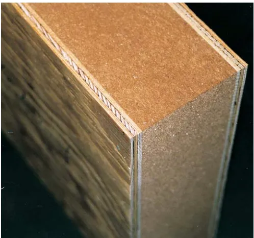
age total thickness of the SW was 96 mm. Hence the core thickness was 78 mm. Figure 1 shows the SW sample. The density profile in the SW core was flat throughout the thick-ness. SW specimens of 260 ⫻ 260 ⫻ 96 mm were prepared for the shear test.
The low-density fiberboard (FB) was manufactured simi-larly, with a core of SW. The target density range for FB was 0.25–0.35 g/cm3
, the same core density as that of SW. The average thickness of the FB was 96 mm. FB specimens of 260 ⫻ 260 ⫻ 96 mm were prepared. Specimens of the raw material of the plywood (PW) were prepared with dimen-sions of 260 ⫻ 260 ⫻ 9 mm.
Shear test method
The shear test method of Japanese Industrial Standard (JIS) A1414 (method A using tie-rods),5
was applied to the
SW, with some modifications of the specimen preparation and apparatus. This method is usually used for full-scale shear wall (i.e., 900 ⫻ 2400 mm or more). A specimen of 260 mm square was regarded as a small shear wall. The test was also applied to PW and FB.
In this connection, there are standard methods for boards.6,8,9
Some studies have been reported, using these methods but they have been on higher density board.10–17
Research using lower-density fiberboard has been slow to evolve.
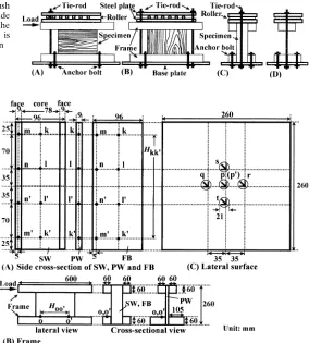
The test conditions are summarized in Table 1. Figure 2 gives the details for preparing the specimen. Four pieces of reinforcing frame of laminated wood (Pseudotsuga menziesii Franco) were glued to both lateral surfaces of the specimen at the top and bottom edges (top and bottom frames) using epoxy resin adhesive. The frame size was 60 ⫻ 60 ⫻ 600 mm. Exceptionally, the width of the bottom frame for PW was 105 mm for convenience so the bolt could be inserted in the same hole as in the other cases (using a frame 60 mm width gives the same results). These frames were also fastened to the specimens for reinforcement using mechanical fasteners such as a lag screw, bolt, nail, and screw nail.
The details of the combination of fastener types used for the top and bottom frames are indicated in Table 1 and Fig. 2. Moderate numbers and sizes of the fastener were selected; they were not excessive to avoid crushing or tear-ing the specimen before loadtear-ing took place. Any of the specimens could provide satisfactory shear deformation corresponding to the applied load. The fasteners could hold the specimen without breaking or being pulled out. The contact area of the fasteners was sufficient even in the fiber materials with larger numbers and sizes.
The outside view of the apparatus of the shear test using tie-rods is illustrated in Fig. 3. The load was applied to the top frames. One tie-rod was used for the monotonic-push (MP) load test (Fig. 3A), and two tie-rods were used for the push-and-pull cyclic (PPC) load test (Fig. 3B). The diameter of the tie-rod was 13 mm. A top-roller and two steel plates piled up over the specimen were fixed lightly to the base plate of steel using the tie-rod. The bottom reinforcing frames were fastened tightly to the base plate with four anchor bolts of 16 mm diameter (Fig. 3C,D). Two adjustable Fig. 1. Sample of the sandwich panel of plywood-overlaid
low-density fiberboard (SW). Total board thickness is 96 mm including a 78 mm thick core and 9 mm thick faces. The density of the specimen is 0.35 g/cm3
Table 1. Test conditions
Sample type Sample Load Tie-rod Direction Fastener type (pieces) Size of lag
(pieces) (pieces)
Top frames Bottom frames
screw (mm)
1 SW (2) MP 1 90° L (5) ⫹ B (1) L (5) 16 ⫻ 150
2 SW (1) MP 1 90° L (5) ⫹ B (1) ⫹ SN (16) L (5) ⫹ SN (12) 16 ⫻ 150
3 SW (1) MP 1 90° L (5) ⫹ B* (1) ⫹ SN (8) ⫹ N (4) L (5) ⫹ SN (4) ⫹ N (8) 16 ⫻ 150
4 SW (4) PPC 2 0° L (10) L (10) 10 ⫻ 100
5 SW (3) PPC 2 90° L (10) L (10) 10 ⫻ 100
6 PW (3) MP 1 0° L (5) B (5) 12 ⫻ 125
7 PW (3) MP 1 90° L (5) B (5) 12 ⫻ 125
8 FB (6) MP 1 – L (5) ⫹ B (1) L (5) 16 ⫻ 150
Direction, setting direction of the sample surface grain to load; MP, monotonic-push load; PPC, push-and-pull cyclic load; L, lag screw; B, bolt (12 ⫻ 240 mm); N, nail (5 ⫻ 150 mm); SN, screw nail (5 ⫻ 150 mm); B*, bolt was connected off sample with frame.
lateral-rollers of 30 mm diameter and 100 mm length made from hard plastic were set aside on the lateral surfaces of the top frames. This was for lateral support to restrict lateral deflection, allowing movement of the specimen along a direction parallel to the applied load direction without frictional restraint.
Two setting directions of the specimen were compared (Table 1): The surface grain of the plywood veneer was taken parallel (0°) or perpendicular (90°) to the applied
load direction for SW and PW. The 90° direction was taken in all cases because it is considered to be more suitable for shear wall. The setting directions are indicated in Fig. 3A,B. For SW, the load test applied was MP for four pieces and PPC for the other seven pieces. For both PW and FB, the MP load test was applied to six pieces each. Although the PPC load test is not yet standardized, it prevails in the field of testing for full-scale shear wall (e.g., for earthquakes). The turning point of the PPC load was considered to occur Fig. 2. Examples of the fastener type (refer to Table 1) indicated in
parentheses for SW (A–C), plywood (PW) (D), and fiberboard (FB) (E). Large circles, L; large squares, B; small circles, N; small squares,
SN. Fasteners were inserted in the frames in front ( filled symbols) and back (open symbols)
Fig. 3. Apparatus of the shear test under the monotonic-push
(A) and push-and-pull cyclic (B) load and its view from the side cross section of SW and FB (C) and PW (D). Examples of the setting direction of the specimen, where the surface grain is parallel (A) or perpendicular (B) to the applied load direction
Fig. 4. Location of the measurement points of the
when the displacement (measured at point k in Fig. 4) indi-cated 1/300, 1/120, 1/60, 1/30, and 1/10 of the sample depth of 260 mm. Loading was continued until complete failure.
Measurement of shear deformation angle
The shear deformation angle of the whole specimen at an early stage must be measured to determine the shear modu-lus. Generally, the standard for a shear wall5
makes it a rule to use a displacement meter, whereas the standard for struc-tural panels8
uses a strain-gauge. With the former method, some displacement meters are set at various places to cover a large portion of the specimen. With the latter method, the strain-gauge covers a relatively limited portion of the speci-men. Such differences in measuring devices and locations are not a problem when the deformation can be assumed to be uniform over the whole material. If it is not uniform, these differences must be taken into consideration.
This problem cannot be avoided for the composite mate-rials of sandwich panels with a low-density core or for lower-density fiberboard. Therefore, in this study shear deformation angles were measured to understand as much of the behavior of SW as possible using both devices (dis-placement meter and strain-gauge). We also examined the differences in their results.
Using the displacement meter
The shear deformation angle of SW was measured using displacement meters, referring to the standard for the wall.5
The location is shown in Fig. 4A,B. Thin plastic plates of 5– 30 mm square were placed on the measurement points. A pair of displacement meters were set horizontally at points k and k⬘ in Fig. 4A at a distance of Hkk⬘. The shear deformation angle including the rotation angle was defined as follows.
γkk δ δ k k
kk
¢
¢
¢ ⫽ ⫺
H (1)
where δk and δk⬘ denote the displacements of the respective points k and k⬘. Another pair of displacement meters were set vertically at points o and o⬘ (Fig. 4B) at a distance of Hoo⬘ on the bottom frame. The rotation angle was defined as follows.
γR δ δ o o
oo
⫽ ⫺ ¢
¢
H (2)
where δo and δo⬘ denote the displacements of the respective points o and o⬘. The shear deformation angle without the rotation angle for the pair of points k and k⬘ was defined as follows.
γk⫽γkk¢⫺γR (3)
For some specimens, another pair of points l and l⬘ were taken to compare with the γk (Fig. 4A). The other two pairs
of points m and m⬘ and points n and n⬘ were taken 5 mm from edge; they were within the face of SW. Similar mea-surements were made for PW and FB.
Using the strain-gauge
The shear deformation angle of SW was measured using a strain-gauge, referring to the standard for the structural panel8
with some modifications of the strain-gauge type and length. The rectangular rosette strain-gauges with a gauge length of 10 mm grid on paper-base with a diameter of 21 mm (K-10-120-B4-11; Kyowa Dengyo Co.) were bonded at the measuring points at the center of both lateral surfaces of the specimen using instant cement. As shown in Fig. 4C, points p and p⬘ were located at the center of each lateral surface of the specimen. The shear deformation angle without rotation angle at point p was determined as follows.
γp⫽2ε45⫺
(
ε0⫹ε90)
(4)where ε0, ε45, and ε90 denote the strain at point p along
directions 0°, 45°, and 90° to the load direction, respectively. The γp⬘ for point p⬘ was determined in the same manner. For some specimens to check with p, another four points (from q to t) were taken on the lateral surface (Fig. 4C). The lateral surface around the measurement points on the face plywood of SW were ground smooth with sandpaper in advance. No knots were found on the surface of the ply-wood. PW was treated similarly. The surface of FB was smooth and hard enough to bond the strain-gauge.
Results and discussion
Evaluation of shear modulus
Shear deformation angle
For SW, the shear deformation angles evaluated using the displacement meter were compared within the pairs of points k to n. The difference between them was not signifi-cant in any specimen. Therefore the value at k was regarded as the representation for each specimen. On the other hand, the shear deformation angles of SW evaluated using the strain-gauge were compared within points p to t. The differ-ence between them was not significant in any specimen. No significant trend was observed. Hence the value at p was regarded as representative for these specimens. Similar trends were observed for PW and FB.
The γk as representive was described again as follows.
γα⫽γk (5)
According to the standard,8
the γp and γp⬘ values were aver-aged and defined as follows.
γ⫽ γ γ ⫹
p p
2
¢
(
)
(6)
The γα values for SW, PW, and FB were defined as γSWα, γPWα, and γFBα, respectively. The γPW, γFB, and γSW values
Load-shear deformation angle curve
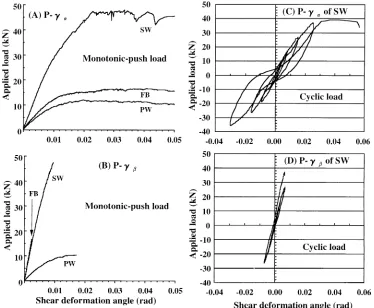
Thus, derived γα and γwere observed in relation to the total applied load, P. Examples of the P/γα and P/γ curves for SW, PW, and FB under the MP load are shown in Fig. 5A and B, respectively. The P/γα and P/γ curves for SW under the PPC load are shown in Fig. 5C and D, respectively.
Under the MP load, the P/γα curves, for each SW, PW, and FB specimen corresponded to the movement of the specimen almost until the final fracture. For each SW speci-men under the PPC load, P/γα gave the typical looping curve, which is usually observed with the wall test.5
The P/
γ data were almost linear in the tests with both types of loading. It followed deformation during the early stage. In the later stage, near the final fracture, the gauge was broken.
Shear modulus of PW and FB
To evaluate the shear modulus of SW, those of PW and FB were investigated first. The slopes of the linear portion of the P/γα and P/γ curves for each specimen were defined as Kα and K, respectively.
Kα P K P
α
⫽ ⫽
γ , γ (7)
The P/γα and P/γdata used in the calculation were within the proportional limits, where the load was less than the P
at the γα was 1/300 radian. The Kα and K values for PW and FB were described as KPWα, KPW, KFBα, and KFB,
respectively.
The Kα and K values for PW and FB in relation to board
density are shown in Fig. 6. The setting direction and fas-tener types are not distinguished in Fig. 6. The effect of the setting direction was not significant. The effect of various fastener types was satisfactorily negligible. In PW (0.68 g/ cm3
), the average value of KPWα was 1.1 MN/rad and that of
KPW was 1.3 MN/rad. In FB the KFBα depended on board
density, and the regression curve of involution function (y
⫽ 34x3.0
, R2 ⫽
0.95, where R2
is correlation coefficient) was fitted (Fig. 6). Hence, the KFBα of FB (0.25–0.35 g/cm3) was
0.5–1.5 MN/rad.
For PW, the GPWα and GPW values were defined as
follows.
G K
A G
K A
PW PW
PW PW
PW PW
α⫽ α, ⫽ (8)
where the APW is the shear sectional area of PW. These
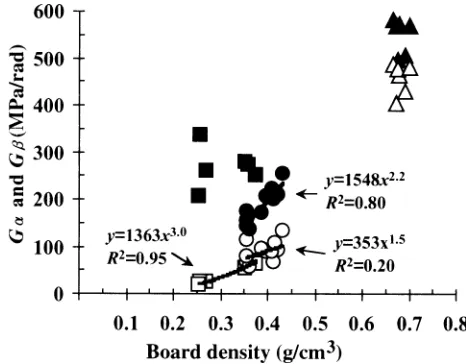
values are shown in Fig. 7. The average GPWα (0.68 g/cm3)
value was 460 MPa/rad, and that of GPW was 550 MPa/rad.
The difference between the GPWα and GPWwas not
significant although GPW was somewhat higher than GPWα.
It was because PW was relatively stiff, uniform material. The shear force transmitted throughout the grain of the veneer effectively over the whole specimen. Hence the measuring location had no effect. The GPWα and GPW
ap-proximated the shear modulus of the entire specimen well.
Fig. 5. Examples of the P–γα and
P–γ curves. The specimens in (A)
For FB, the GFBα and GFB values were defined similarly.
G K
A G
K A
F F
FB F
F FB
Bα⫽ Bα, B⫽ B (9)
where the AFB is the shear sectional area of FB. A difference
between GFBα and GFB was observed: GFB was much higher
than GFBα. The GFBα was dependent on the board density.
The GFBα increased with the increase in board density. The
GFBα at densities of 0.25, 0.30, and 0.35 g/cm3 were 21, 37,
and 58 MPa/rad, respectively, according to the regression curve (y ⫽ 1363x3.0
, R2⫽
0.95) (Fig. 7). According to Wong,18
the shear modulus of fiberboard with a density of 0.3–0.4 g/cm3
evaluated by the torsion method is 30–36 MPa, and that of particleboard (0.3–0.4 g/ cm3
) evaluated by the tapping method is 22–96 MPa. Com-pared to these results, the GFBα is considered to be highly
reliable as the shear modulus of FB. GFB seemed
indepen-dent of board density and was around 200–300 MPa/rad (Fig. 7). This value is high considering the low board density.
One reason is the construction of FB with low-density fiberboard, which is a uniform fibrous material. The shear force transmitted effectively throughout the specimen through the many contact points of a large number of fibers. Shear deformation was elastic during the early stage and seemed uniform macroscopically. No local fractures were observed, although it is possible that there were micro-scopic local fractures that caused the whole deformation. The limited measured location remained stable compared to the overall behavior. Hence GFBwas negligible for the
purpose of this study. Further investigation of the distribu-tion of shear deformadistribu-tion within a fiberboard is left to fu-ture studies.
Evaluation of the shear modulus of SW
The KSWα and KSW values are shown in Fig. 6. There was a
difference between them. Both values depended strongly on board density (core density), unlike FB. According to the regression curves fitted for KSWα (y ⫽ 8.7x1.5, R2⫽ 0.20)
and KSW (y ⫽ 38x2.2, R2⫽ 0.80), the KSWα was 1.8–2.2 MN/
rad, and the KSW was 3.8–5.1 MN/rad for the density range
0.35–0.40 g/cm3
(Fig. 6).
The differences between KSWα and KSW were derived
from the difference between γSWα and γSW. As discussed
above, the shear deformation angles measured in a section of the face were the same as those of the core but were different from those on the surface of the face. The differ-ence was seen in the face materials. Location had no effect in a specimen of plywood only. One reason for this was the sandwich construction, with two stiff faces and a fibrous core. Under shear force these elements behaved neither together nor independently. Such an interaction made the behavior of SW, as a composite, unique.
The hypotheses should be examined theoretically. For example, there is a method for calculating the divided shear force in the horizontal diaphragm (floor or ceiling between shear walls) when designing wooden house construction.19
It deals with rigid and flexible floors. Therefore, it is set up for sandwich panel construction so the shear modulus of SW can be analyzed.
Analysis of the shear modulus of SW
To understand the shear behavior of SW, the measured values of γSWα and γSW are regarded as partial contributors.
To examine their contribution to the overall behavior, some experimental models are proposed. Experimental shear moduli can be derived from each model. On the other hand, a theoretical model using the shear moduli of PW and FB can be calculated. These values are compared, and it can be determined which experimental model more accurately simulates SW behavior.
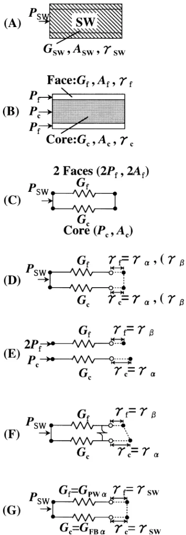
To examine the relation between deformation and shear force in the shear section, models of SW shear sections are considered (Fig. 8). The factors of load (P), shear modulus Fig. 6. Values of Kα (open symbols) and K (filled symbols) of SW
(circles), PW (triangles), and FB (squares) in relation to the board density. Solid lines, regression curves for KSWα, KSW, and KFBα
Fig. 7. Values of Gα (open symbols) and G (filled symbols) of SW
Pc⫽G Ac c cγ (11)
Psw⫽ ⫹Pc 2Pf (12)
Experimental models of SW
The experimental shear modulus of SW was evaluated first. The spring model is considered (Fig. 8C). It consists of two elastic springs; one indicates the two faces and the other indicates the core. Factors 2Pf, Gf, 2Af, and γf are assigned
to the two faces. Factors Pc, Gc, Ac, and γc, are assigned to
the core. The relations between the values for γc and γf and
the measured values for γSWα and γSW are assumed as
follows.
γc⫽γSWα,γf⫽γSWα (13)
γc⫽γSW,γf⫽γSW (14)
γc⫽γSWα,γf⫽γSW (15)
Equations 13 and 14 indicate that the effect of the measur-ing location is ignored in the shear section. They assume that SW is rigid material, and that the rigid model is derived (Fig. 8D). The location effect is considered in Eq. 15, where SW is assumed to be rather flexible, and the flexible model (Fig. 8E) and semirigid model (Fig. 8F) are derived from it. The γSWα and γSWvalues are regarded as partial to some
extent. To evaluate the GSW for each model, Gc and Gf are
calculated. Gc can be obtained from Eqs. 10–12.
G P G A
A
c
SW f f f c c
⫽ ⫺2 γ
γ (16)
The Gc and Gf values for each model are derived as follows.
Rigid model. When it is supposed that the composite be-haves like a completely unified rigid material, the “rigid model” is proposed (Fig. 8D). In the “rigid model” the shear deformations of the elements correspond completely (Eqs. 13 and 14). The rigid models based on Eqs. 13 and 14 are called the “rigid-α model” and the “rigid- model,” respectively. They satisfy Eq. 17.
γc⫽γf (17)
The Gc based on Eqs. 13 and 14 is defined as GcRα and GcR,
respectively. From Eq. 16,
G K G A
A
cR
SW f f c
α⫽ α⫺2 (18)
G K G A
A
cR
SW f f c
⫽ ⫺
2
(19)
The Gf values in these models are taken to be 460 MPa/rad
considering GPWα.
Flexible model. When it is supposed that each element of the core and face behaves separately and independently, Fig. 8. Models of shear section of SW. Diagrams of the composite body
(A) and elements (B). Spring models of basic (C) and experimental models [rigid (D), flexible (E), and semirigid (F) models] and of the theoretical model (G)
(G), shear area (A), and shear deformation angle (γ) are assigned to SW as a composite (Fig. 8A) and its elements (Fig. 8B), respectively. Subscript SW indicates the com-posite body of SW, and subscripts c and f indicate the core and one of the faces, respectively. Generally,
the “flexible model” is proposed (Fig. 8E). In the “flexible model” it is supposed that the shear deformations of the elements are different (Eq. 15), and that the portion of load is in proportion to the shear sectional area (Eqs. 20 and 21).
P P A A
c
SW c SW
⫽ (20)
P P A A
f
SW f SW
⫽ (21)
The Gc value obtained from Eqs. 11 and 20 is defined as GcF.
G K
A
cF SW SW
⫽ α
(22)
In this model Gf is calculated from KSW divided by ASW. It is
144–255 MPa/rad.
Semirigid model. When it is supposed that the behaviors of the elements are not the same but are dependent on each other, the “semirigid model” is proposed (Fig. 8F). The dependent interaction between the faces and core is ex-pressed as the shear spring in Fig. 8F. In the “semirigid model” it is supposed that the shear deformations of the core and face are different based on Eq. 15. The Gc
obtained from Eq. 16 is defined as GcS.
G
G A K
A K
cS
f f SW c
SW
⫽ ⫺
1 2 1
1
α
(23)
In this model the Gf value is taken to be 460 MPa/rad.
Shear modulus of the core
Each Gc is examined if it approximates the shear modulus of
fiberboard. The core density is 0.28–0.33 g/cm3
for SW with a board density of 0.35–0.40 g/cm3. The GcRα, GcR, GcF, and
GcS are shown in relation to the core density of SW in Fig. 9.
The values of Gc depend on the core density. The regression
curves (solid lines) were fitted for GcRα (y ⫽ 306x ⫺ 93, R2⫽
0.18), for GcR (y ⫽ 3150x2.9, R2⫽ 0.78), for GcF (y ⫽ 266x 0.97
, R2⫽
0.19), and for GcS (y ⫽ 824x 2.4
, R2⫽
0.50). The shear modulus is thought to depend increasingly on board density similarly to the other mechanical board properties. There-fore the involution function was applied. A straight line was fitted to GcRα instead, as it included a minus value.
Accord-ing to the curves (0.28–0.33 g/cm3
), GcRα ranges from ⫺7 to ⫹8 MPa, though the minus value is impossible; GcR is 79–
126 MPa/rad; GcF is 77–91 MPa/rad, and GcS is 39–58 MPa/
rad, as shown in Table 2.
The GFBα is given in relation to the density of FB (dashed
line, y ⫽ 1363x3.1
, R2⫽
0.95). GFBα is 30–49 MPa/rad at the
density range. The value of Gc was compared with that of
GFBα. GcRα is less than 16% of GFBα. GcR is 260%. GcF is
190%–260%. GcS is 120%–130%. Therefore, GcS is nearest
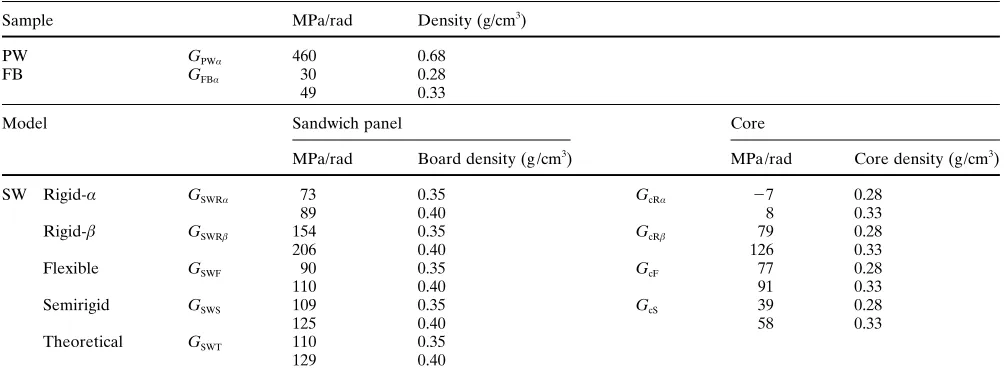
Table 2. Results of the analysis of shear modulus of SW
Sample MPa/rad Density (g/cm3)
PW GPWα 460 0.68
FB GFBα 30 0.28
49 0.33
Model Sandwich panel Core
MPa/rad Board density (g /cm3) MPa/rad Core density (g/cm3)
SW Rigid-α GSWRα 73 0.35 GcRα ⫺7 0.28
89 0.40 8 0.33
Rigid- GSWR 154 0.35 GcR 79 0.28
206 0.40 126 0.33
Flexible GSWF 90 0.35 GcF 77 0.28
110 0.40 91 0.33
Semirigid GSWS 109 0.35 GcS 39 0.28
125 0.40 58 0.33
Theoretical GSWT 110 0.35
129 0.40
PW, plywood; FB, thick, low-density fiberboard; SW, wood-based sandwich panel of plywood-overlaid low-density fiberboard; G, shear modulus
to GFBα. These values are examined again together later
with GSW.
Experimental shear modulus of SW
Using each pair of Gc and Gf obtained in the above, GSW for
each model is calculated on the basis of the strain energy stored in the whole specimen. Under the proportional limit, the strain energy U is
U P P D
GA
⫽ δ⫽
2 2
2
(24)
where D denotes the depth of the specimen. There is the following relation for a sandwich panel.
USW⫽Uc⫹2Uf (25)
where the USW, Uc, and Uf denote the U of a sandwich panel,
core, and a face, respectively. Substituting Eq. 24 for Eq. 25, and from Eqs. 10 and 11, GSW is derived as follows.
G
A G A P
G A P
SW SW
c c c SW
2
f f f SW 2 ⫽ ⫹ 1 2 2 2 γ γ Ê Ë Á ˆ ¯ ˜ (26)
The GSW for each experimental model is derived as follows.
In the rigid-α model Eq. 26 becomes
G
A G A
K G A K SWR SW cR c SW 2 f f SW 2 α α α α ⫽ ⫹ 1 2 Ê Ë Á ˆ ¯ ˜ (27)
where GSWRα denotes the GSW in the rigid-α model. For the
other models, the GSW are defined as follows.
G
A G A
K G A K SWR SW cR c SW 2 f f SW 2 ⫽ ⫹ 1 2 Ê Ë Á ˆ ¯ ˜ (28) G
A G A
K G A K SWF SW cRF c SW 2 f f SW 2 ⫽ ⫹ 1 2 α Ê Ë Á ˆ ¯ ˜ (29) G
A G A
K G A K SWS SW cRS c SW 2 f f SW 2 ⫽ ⫹ 1 2 α Ê Ë Á ˆ ¯ ˜ (30)
where the GSWR, GSWF, and GSWS denote GSW in the rigid-,
flexible, and semirigid models, respectively. The GSWRα and
GSWR values are consequently defined in Eq. 31.
G P A G P A SWR SW SW SWR SW SW α α ⫽ ⫽
γ , γ (31)
These GSWRα, GSWR, GSWF, and GSWS values are shown in Fig.
10. As they depended increasingly on board density, the regression curves (solid lines) of involution function were
fitted for GSWRα (y ⫽ 353x1.5, R2⫽ 0.20), GSWR(y ⫽ 1548x2.2,
R2 ⫽
0.80), GSWF (y ⫽ 435x 1.5
, R2⫽
0.20), and GSWS (y ⫽
312x1.0
, R2⫽
0.22). According to these curves, the values of GSWRα (0.35 and 0.40 g/cm3
) are 73 and 89 MPa/rad (Table 2); those of GSWR are 154 and 206 MPa/rad; those of GSWF are
90 and 110 MPa/rad; and those of GSWS are 109 and 125 MPa/
rad, respectively.
Theoretical model of SW
To calculate the theoretical shear modulus of SW, consider the theoretical model (Fig. 8G), where it is assumed that:
γc⫽ ⫽γf γSW (32)
Generally,
PSW⫽GSWASWγSW (33)
Using Eqs. 16, 32, and 33, the theoretical shear modulus of SW is defined as GSWT.
G G A G A
A
SWT
c c f f SW
⫽ ⫹2 (34)
The values of GFBα and GPWα (460 MPa/rad) are substituted
for Gc and Gf in Eq. 24, respectively. Then the GSWT is
calculated, and the regression curve of involution function is fitted to GSWT (y ⫽ 387x
1.2
, R2 ⫽
0.95, dashed line), as shown in Fig. 10 in relation to the calculated board density of SW. Accordingly, GSWT is 110–129 MPa/rad at a density
range of 0.35–0.40 g/cm3
.
Comparison with theoretical shear modulus of SW
The GSWRα, GSWR, GSWF, and GSWS values (solid lines) are
compared with GSWT (y ⫽ 387x 1.2
, R2⫽ 0.95, dashed line) in Fig. 10. GSWT is 110 and 129 MPa/rad (0.35 and 0.40 g/cm
3
0.40 g/cm3
, GSWRα is 67% and 69% of GSWT, respectively, and
GSWR is 140% and 160%. GSWF is 82% and 85%, and GSWS is
99% and 97%.
The above results are summarized considering both GSW
and Gc. The rigid-α model gives moderate simulation,
be-cause GSWRα is about 70% of GSWT, and GcRα is less than 16%
of GFBα. The rigid- model is not appropriate because GSWR
values are 140%–160% of GSWT, and GcR is 260% of GFBα.
In the flexible model, GSWF is nearer GSWT (more than 80%
of GSWT), but it is an imbalance that GcF is 190%–260% of
GαFB, and GfF was much lower than GPW. The semirigid
model gave the closest simulation, because GSWS
approxi-mates GSWT (almost 100% of GSWT), and GcS is closest to
GFBα (120%–130% of GFBα).
As a result, the measured values of γSWα and γSW gave
major and local contribution to the overall behavior, re-spectively, in SW. The shear behavior of SW was similar to that of the rigid-α model basically. The semirigid model was a better approach when taking local behavior into consider-ation, as it gave a closer approximation to the theoretical value. Further investigation of the interaction between the core and faces will be helped by determining the partial distribution of loading and its profile within SW.
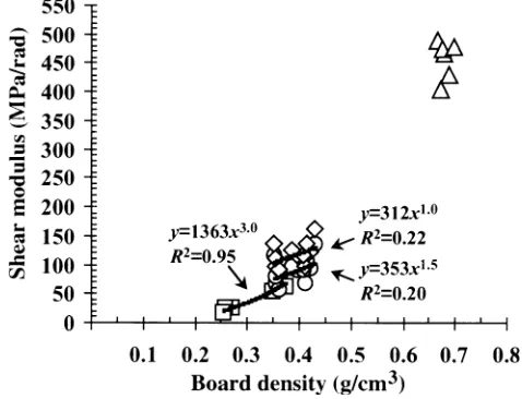
Shear modulus of SW
The shear moduli of PW and FB were evaluated by GPWα
and GFBα, respectively, as shown in Fig. 11. The shear
modu-lus of PW (0.68 g/cm3
) was 460 MPa/rad, and that of FB (0.25–0.35 g/cm3
) was 21–58 MPa/rad.
The GSWRα and GSWS values are shown in Fig. 11 as the
experimental shear modulus of SW. According to the re-gression curves of GSWRα and GSWS (solid lines), the
experi-mental shear moduli of SW (0.35–0.40 g/cm3
) were 73–89 and 109–125 MPa/rad, respectively. The theoretical shear modulus of SW (0.35–0.40 g/cm3) was 110–129 MPa/rad. Based on GSWRα and GSWS, respectively, the shear moduli of
SW are about 1.8–2.4 times and 2.6–3.7 times higher than that of the core, referring to GFBα (0.28–0.33 g/cm3, 30–
49 MPa/rad).
In this connection, the calculated shear modulus of the structural panel composite, which consists of a pair of nailed structural plywood specimens of 9 mm thickness with a full-scale shear wall size, is 106 MPa/rad.20
The shear modulus of SW matches it, though they cannot be com-pared exactly.
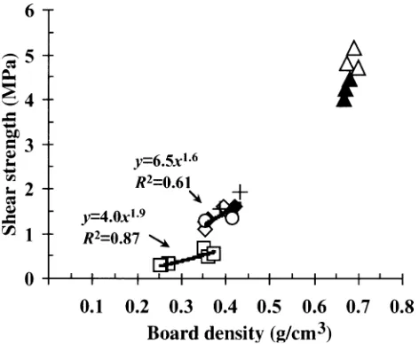
Shear strength
Figure 12 shows a typical shear failure appearance of SW. Shear failure occurred in all of the other specimens of SW as well as PW and FB.
The shear strength (τ) of SW was defined as the maxi-mum load divided by the shear area. The τ is indicated in relation to board density in Fig. 13. The effect of the setting direction on τ was not significant. The effects of the fastener type on τ were negligible. There was no reduction of the τ value for SW under the PPC load compared to that under
Fig. 11. Experimental shear moduli of SW evaluated by GSWRα (open
circles) and GSWS (open diamonds), compared with the shear moduli of PW and FB evaluated by GPWα (open triangles) and GFBα (open
squares), respectively. Solid lines, regression curves for GSWRα, GSWS, and GFBα
Fig. 12. Example of the ultimate stage of shear failure of SW. The
direction of the surface grain of the face plywood is perpendicular to the loading direction. The density of the specimen is 0.41 g/cm3. Both face and core were crushed by the shearing stress. The fracture occurred around the neutral surface of the test specimen
the MP load. A similar trend was observed in the τ values for PW and FB.
Without recognizing the setting direction and fastener type, the trends can be summarized as follows. As the τ of SW depended on board density, the regression curve of involution function was fitted to SW ( y ⫽ 6.5x1.6
, R2⫽ 0.61). According to this calculation, the τ of SW (0.35–0.40 g/cm3
) was 1.2–1.5 MPa. The average τ of PW (0.68 g/cm3
) was 4.6 MPa. As the τ of FB depended on board density, the regression curves of involution function were fitted ( y ⫽ 4.0x1.9
, R2⫽
0.87). Therefore, the τ of FB (0.25–0.35 g/cm3
) was 0.29–0.54 MPa.
The τ of SW at densities of 0.35 and 0.40 g/cm3
were 3.4 and 3.1 times higher than those in the core, with densities of 0.28 and 0.33 g/cm3
Fig. 13. Shear strength of SW (open circles, type 1; crosses, types 2, 3;
filled diamonds, type 4; open diamonds, type 5), of PW ( filled triangles, type 6; open triangles, type 7), and of FB (open squares, type 8). Solid lines, regression curves for SW and FB. Refer to Table 1 for the fastener type
Conclusions
The shear test method using tie-rods for the general shear wall was useful for investigating the fundamental shear be-havior of SW as a small shear wall. The shear modulus must be carefully determined in low-density fiberboard and sand-wich panels. Knowledge about the shear behavior of SW can provide a basis for the development of wood-based sandwich panels as practical shear walls.
Acknowledgments The authors express our deep gratitude to Mr.
Noritoshi Sawada (Hokushin Co.), Dr. Wong Cheng, and their coop-erative members for their expert technical support for the preparation of manufacturing the thick fiberboard and sandwich panel. We are grateful also to Drs. Min Zhang, Kenji Umemura, Wong Ee Ding, and Guangping Han for their great help and advice in manufacturing the thick panels. The authors are grateful to Hokushin Co. for the fiber and resin and to Ishinomaki Gouhan Co. for the plywood. We thank Mr. Makoto Nakatani for his expert assistance when preparing the speci-mens for the shear test. Funding provided by the Research Fellowship of the Japan Society for the Promotion of Science for Young Scientists as a JSPS Research Fellow is also gratefully acknowledged.
References
1. Jack RV (1999) The behavior of sandwich structures of isotropic and composite materials. Technomic Publishing, Lancaster, PA, USA
2. Gibson LJ, Ashby MF (1997) The design of sandwich panels with foam cores. In: Clarke DR, Suresh S, Ward FRSIM (eds) Cellular solids. Cambridge University Press, Cambridge
3. Kawasaki T, Zhang M, Kawai S (1998) Manufacture and proper-ties of ultra-low density fiberboard. J Wood Sci 44:354–360 4. Kawasaki T, Zhang M, Kawai S (1999) Sandwich panel of
veneer-overlaid low-density fiberboard. J Wood Sci 45:291–298
5. Japanese Industrial Standard (1994) JIS A 1414–1973 Methods of performance test of panels for building construction. Japanese Standard Association, Tokyo
6. Japanese Agricultural Standard (1999) JAS for structural plywood. Ministry of Agriculture, Forestry and Fisheries, Tokyo
7. Sasaki H (1990) Development of continuous press with steam-injection heating from both sides. Report of the grants-in-aid for scientific research (no. 01860023) from the Ministry of Education, Science and Culture, Japan
8. American Society of Testing and Materials (1996) D2719-89 standard test methods for structural panels in shear through-the-thickness. In: 1996 Annual book of ASTM standards. ASTM, Philadelphia
9. American Society of Testing and Materials (1996) D1037-96 stan-dard test methods for evaluating properties of wood-base fiber and particle panel materials. In: 1996 Annual book of ASTM stan-dards. ASTM, Philadelphia
10. Okuma M (1961) Shearing modulus of plywood and hardboard measured by the panel shear test. I. Measuring of shearing modu-lus by the ASTM method (in Japanese). Mokuzai Gakkaishi 7:242– 246
11. Okuma M (1962) Shearing modulus of plywood and hardboard measured by the panel shear test. II. Investigations on the form of the load-strain curve (in Japanese). Mokuzai Gakkaishi 8:54–58 12. Okuma M (1962) Shearing modulus of plywood and hardboard
measured by the panel shear test. III. Measuring of shear modulus by the improved Larsson-Wästlund method (in Japanese). Mokuzai Gakkaishi 8:58–61
13. Takami I (1964) Panel and plate shear test for plywood (in Japanese). Mokuzai Gakkaishi 10:1
14. Sasaki H, Maku T (1964) Strain distribution on plywood panel shear test specimens (in Japanese). Mokuzai Kenkyu 33:37–46 15. Okuma M, Shida S, Ohhashi M (1983) Manufacture and
perfor-mance of radiata pine plywood. I (in Japanese). Mokuzai Gakkaishi 29:438–443
16. Suzuki S, Nawa D, Miyamoto K, Shibusawa T (2000) Shear-through-thickness properties of wood-based panels determined by the two-rail shear and edgewise shear methods. J Soc Mater Sci 49:395–400
17. Lee AWC, Stephens CB (1988) Comparative shear strength of seven types of wood composite panels at high and medium relative humidity conditions. For Prod J 38(3):49–52
18. Wong ED (1999) Density profile: its formation and effects on the properties of particleboard and fiberboard. Dissertation, Depart-ment of Forest and Biomass Science, Graduate School of the Faculty of Agriculture, Kyoto University, pp 69–70
19. Nihon Jutaku Mokuzai Technical Center (1989) The information for the design of the three-storied wooden house construction and fire resistance (in Japanese). Ministry of Construction, Tokyo, pp 15–21