ORIGINAL ARTICLE
Hiroaki Nagai · Koji Murata · Takato Nakano
Defect detection in lumber including knots using bending defl ection curve:
comparison between experimental analysis and fi nite element modeling
Abstract A new method has been developed for detecting
localized defects such as edge knots using a bending defl ec-tion curve. The coordinates of a bottom edge (edgeline) of an unloaded piece of lumber are extracted from a digital image, and a bending defl ection curve is obtained from the displacement of the edgeline of the lumber using a digital image correlation (DIC) technique. Depending on the knots within the beam, the bending defl ection curve is shifted from the curve of a defect-free beam. The measured bending defl ection curve is regressed to a theoretical curve by elementary beam theory. A fi nite element method (FEM) model of the beams including defects as simplifi ed knot structure has been performed. Comparison between the bending experiment and FEM analysis shows that cross-sectional reductions cause characteristic variations in the bending defl ection curves depending on the position of encased knots, and local grain distortions cause variations in the curves depending on the direction of spike knots. Using the residual variance between the measured defl ec-tion curve and a polynomial regression curve, it is possible to detect knots at which failures initiate.
Key words Bending defl ection curve · Defect detection ·
Knot · Digital image correlation
Introduction
Lumbers usually contain defects such as knots and fi ber deviations in the vicinity of knots. The presence of these defects strongly affects the strength and stiffness of lumbers.
H. Nagai (*) · K. Murata · T. Nakano
Division of Forest and Biomaterials Science, Graduate School of Agriculture, Kyoto University, Kitashirakawa Oiwake-cho, Sakyo-ku, Kyoto 606-8502, Japan
Tel. +81-75-753-6236; Fax +81-75-753-6300
e-mail: [email protected]
Part of this article was presented at the 57th Annual Meeting of the Japan Wood Research Society, Hiroshima, Japan, August 2007
Because knots are regarded as the major strength-reducing defects, studies to consider the effect of knots and the fi ber deviations in the vicinity of knots on the strength of lumbers have been carried out by many researchers (e.g., Mitsuhashi et al.1
).
In past decades, a large number of studies have been performed in the fi eld of nondestructive testing of wood. In these studies, many physical properties of lumbers have been used for the detection of knots. For example, the optical properties of a lumber surface such as color and
gloss have been employed.2,3
Furthermore, several
auto-mated visual inspection systems have been developed.4,5
However, optical information does not directly refl ect the mechanical properties of the defects. Using X-rays or gamma rays, the density distribution in lumbers can be
determined.6,7
Radiation techniques are based on the fact that knots have a higher density than the surrounding
mate-rial. In research conducted by Boström,6 the size, location,
and even the shape of knots were obtained. Thermographic measurements have also been employed for the detection
of knots and the slope of grains in lumbers.8
Thermal methods are based on the differences in the thermal con-ductivity and the heat absorption of knots and the sur-rounding material. Among other methods employed for the detection of knots, an ultrasonic sound technique based on
longitudinal stress wave speed9 and a microwave technique
using a microwave scanner have been developed. In partic-ular, microwave techniques are being seriously considered
for machine grading systems.10,11
Although these methods have produced good results on a laboratory scale, it will be diffi cult to achieve cost effi ciency if these methods are intro-duced in small mills in Japan.
To study the mechanical properties of a lumber effec-tively, its response to a mechanical stimulus has to be observed. The most widely applied machine grading prin-ciple is to measure the bending modulus of elasticity (MOE) of lumbers. If a lumber contains a serious defect, the bending defl ection curve may deviate from the theoretical curve.
Murata et al.12
measured the strain distribution in the vicin-ity of a knot by a four-point bending test using a digital image correlation (DIC) technique. In the present study, a Received: May 28, 2008 / Accepted: December 4, 2008 / Published online: February 20, 2009
bending defl ection curve was measured using the DIC tech-nique, which yielded the subpixel displacement of the points under consideration using a correlation function and inter-polation among pixels. The purpose of this study was to detect the localized defects in lumber including knots, at which failures initiate, by using the bending defl ection curves.
Theory
When a wooden beam is loaded at the center of its span, its defl ection y can be expressed by the elementary beam theory as follows:
y P
EI x L x
P EIx
PL EIx
= −
(
−)
= − +48 4 3 12 16
3 2 3
2
(1)
where E is Young’s modulus, I is the geometrical moment of inertia, L is the span length, P is the load at midspan, and x is the distance from the supporting point. In this study, Eq. 1 is regarded as a theoretical curve. The mea-sured bending defl ection coordinates are regressed to Eq. 2 at a given interval. Equation 2 is of the same form as Eq. 1.
y=αx3+βx (2)
If a regression region on the beam defl ection curve includes a knot, the obtained curve changes characteristi-cally. The change can be estimated in the following manner. First, it is expected that a knot breaks the local bending stiffness EI of the wooden beam. From Eqs. 1 and 2, EI can be calculated as follows:
EIα= − Pα EIβ=PLβ
12 16
2
, (3)
where EIa and EIb are obtained from the coeffi cients a or
b in Eq. 2. Second, a knot distorts the grains in its vicinity,
and the edge of the distorted region expands or shrinks along the direction of the beam height. To evaluate the deviation from the theoretical curve, a residual variance is obtained. The residual variance is the variance of the square sum of the difference between the measured defl ection curve and the polynomial regression curve.
Experimental
Defect detection using static bending test
Twenty-one pieces of commercial 38 × 89 mm SPF lumber
were used as specimens. The specimens were not identifi ed with regard to species. Nondestructive three-point and destructive four-point bending tests were performed using a universal testing machine (Shimadzu; capacity, 98 kN) at
a crosshead displacement speed of 5 mm min−1
.
The three-point bending test was carried out with a span length of 1400 mm. The maximum applied load was 1.5 kN, which was suffi ciently smaller than the estimated rupture
load, because the modulus of rupture (MOR) for a clear
spruce specimen was assumed to be 75 MPa.13
The bending defl ection curve was calculated as follows, which was the same method as described in previous report.14
The deformation in the beam specimens was recorded by using two digital still cameras (Nikon D100; Zoomnikkor 105 mm) when a load of 1.5 kN was applied. The photographed region was on the left side of the
speci-men. The image size was 3008 × 2000 pixels. Each pixel was
approximately equal to 0.15 × 0.15 mm2
(the dimensions of
the observed fi eld were approximately 450 × 300 mm2
for each camera). The coordinates of a bottom edge (edgeline) of an unloaded specimen were obtained from the digital image by using image processing techniques: Otsu binariza-tion15
and edge detection techniques. The deformation at the edgeline was measured using in-house DIC software that yielded the subpixel displacement of the points under consideration using a correlation function and interpolation among the pixels. The defl ection under a load of 0.2 kN was defi ned as the base defl ection of the unloaded specimen to exclude the initial twist in the specimen during the measurements.
The measured bending defl ection coordinates were regressed to Eq. 1 at the given interval (50 mm) and the coeffi cients were calculated using a polynomial regression. Because the interval affects the accuracy of defect detec-tion, the sampling interval was experimentally determined in the previous analysis.
The destructive four-point bending test was performed with a loading span of 540 mm and a supporting span of
1620 mm at a crosshead displacement speed of 5 mm min−1
. The deformation in the beam specimen was recorded in the same manner as in the three-point bending test.
Study by fi nite element modeling (FEM) simulation
In the past few decades, studies concerning FE modeling of solid wood including knots have been performed by several wood research groups. For example, FE analyses based on linear fracture mechanics have been performed by a research
group at Colorado State University.16–18
In these models, the
fl ow-grain analogy19
was utilized to account for a localized grain deviation associated with knots. Another research group at Vienna University of Technology introduced a multisurface plasticity model for clear wood in
consider-ation of elasto-plastic material20
and this was applied to
consider the effect of knots.21
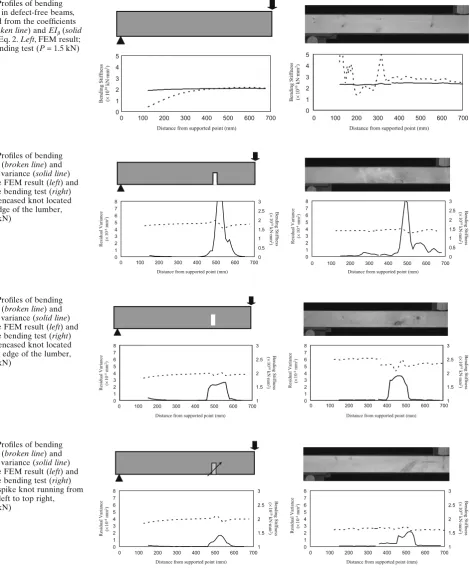
of knots, for example, encased knots and spike knots. Figure 3 shows the measured bending defl ection curve and the polynomial regression curves. The residual variance between the measured defl ection curve and the polynomial regression curve in regions with knots was found to be higher than that for knot-free regions.
Figure 4 shows the EI profi les of the defect-free beams obtained from the coeffi cients of the polynomial regression curve at the given interval (50 mm). In the case of the defect-free beams, EI should have the same value. Devia-tion of the broken line near the origin appears to be caused by the effect of stress concentration at the supporting or
loading point. In a comparison of EI profi les, EIa enhances
irregular factors. In order to avoid such effects, EIb is used
to identify the local bending stiffness EI in this study. Figures 5 and 6 illustrate the profi les of EI and residual variance including the region with encased knots. Figure 5 shows a lumber including an encased knot that is located at the bottom edge (Type 1). The distance from the gap to the bottom edge is 0 mm in the FEM model (left side of Fig. 5). Figure 6 shows a lumber including an encased knot that is located near the bottom edge (Type 2). The distance from the gap to the bottom edge is 2.5 mm in the FEM model (left side of Fig. 6). Both the EI and residual variance pro-fi les obtained from the experimental and FEM analyses exhibit similar patterns, as shown in Figs. 5 and 6. Compari-son of the two profi les shows that the residual variance profi le exhibits the characteristic pattern more clearly. The residual variance increases with the tangential length of the gap and a decrease in the distance from the edge of the specimen. It is concluded that the cross-sectional reductions
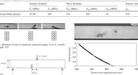
Fig. 1. Rotation of axis of elements (material angle). Left, 0°; middle,
45°; right, 135°
180 mm
1400 mm P = 1.5 kN
90 mm
L T
Table 1. Specimen properties for fi nite element analysis
Specimen Young’s modulus Shear modulus Poisson ratio
EL (MPa) ET (MPa) GLT (MPa) GLR (MPa) GRT (MPa) mLT
Clearwood (Sitka spruce) 10 700 430 618 500 43 0.51
Fig. 2. Finite element method (FEM) model of the three-point bending
test
Distance from supported point (mm)
Deflection (mm)
2 2.2 2.4 2.6 2.8 3
300 400 500 600 700
the regions with the spike knots, the grains in the vicinity of these knots ran from bottom left to top right (45°) or from bottom right to top left (135°).
A two-dimensional model of a wooden beam was simu-lated by using MSC/NASTRAN ver. 70.0 (Fig. 2). The beam was modeled with four node orthotropic linear ele-ments and it was assumed that the eleele-ments deform as perfect elastic bodies. All the elements had a constant size
of 0.625 (L) × 1.25 (T) mm, and the dimensions of the cross
section of the beam model were 90 (T) × 40 (R) mm. Its
span length was 1400 mm. The applied load to calculate bending defl ection curves was 1.5 kN. The supporting point on one side was allowed to move along the x-axis (longitu-dinal direction) and was rotated freely around the z-axis (radial direction). The material properties of clear wood are listed in Table 1.
The defects were arrayed at a distance of 520 mm from the supporting point. The dimensions of the gap were 2.5
(L) × 20 (T) mm, and the dimensions of the region where
the material angle was modifi ed were 10 (L) × 20 (T) mm.
The displacement of the nodes at the bottom edge was defi ned as the defl ection curve. These bending defl ection curves were analyzed by using the same method as that for digital imaging analysis, stated above.
Results and discussion
The bending defl ection curves across the knots were found to be characteristically distorted according to the types
Fig. 3. Measured bending defl ection curve (gray line) and polynomial
cause the characteristic variations in the bending defl ection curve observed at the encased knots.
The profi les of EI and residual variance including the region with spike knots are presented in Figs. 7 and 8. The material angles are 45° (Type 3) and 135° (Type 4) in Figs. 7 and 8, respectively. Elements with a material angle of 0° are regarded as defect-free materials. The experimen-tal profi les display characteristic patterns similar to the FEM
profi les shown in Figs. 7 and 8. The profi les of the residual variance exhibit the characteristic pattern more clearly than those of EI. When other FEM models with different mate-rial angles (15°, 30°, 60°, 90°, etc.) were analyzed, it was found that the peak of the residual variance profi le shows the maximum value for the material angles of 45° and 135°. The local grain distortion caused by spike knots infl uences the bending defl ection curves. These results show that the 0 1 2 3 4 5 0
Distance from supported point (mm)
Bending Stiffness (×
10
10 kN·mm 2) 700 600 500 400 300 200 100 0 1 2 3 4 5
Bending Stiffness (×
10
10
kN·mm
2)
0
Distance from supported point (mm)
700 600 500 400 300 200 100
Fig. 4. Profi les of bending
stiffness in defect-free beams, obtained from the coeffi cients
EIa (broken line) and EIb (solid
line) in Eq. 2. Left, FEM result;
right, bending test (P = 1.5 kN)
0 1 2 3 4 5 6 7 8 0 0 0.5 1 1.5 2 2.5 3
Distance from supported point (mm)
Residual Variance
(
×
10
-4 mm 2) Bending Stiffness ( × 10 10 kN·mm 2 ) 700 600 500 400 300 200 100 Residual Variance ( × 10
-4 mm 2) Bending Stiffness ( × 10 10 kN·mm 2 ) 0 1 2 3 4 5 6 7 8 0 0.5 1 1.5 2 2.5 3
Distance from supported point (mm)
0 100 200 300 400 500 600 700
Fig. 5. Profi les of bending
stiffness (broken line) and residual variance (solid line) from the FEM result (left) and from the bending test (right) (type 1 encased knot located at the edge of the lumber,
P = 1.5 kN)
Distance from supported point (mm) Residual Variance (
× 10 -4 mm 2) Bending Stiffness ( × 10 10 kN·mm 2 ) 0 1 2 3 4 5 6 7 8 0 1 1.5 2 2.5 3 700 600 500 400 300 200 100 Residual Variance ( × 10 -4mm 2) Bending Stiffness ( × 10 10 kN·mm 2 )
Distance from supported point (mm)
0 1 2 3 4 5 6 7 8 1 1.5 2 2.5 3
0 100 200 300 400 500 600 700
Fig. 6. Profi les of bending
stiffness (broken line) and residual variance (solid line) from the FEM result (left) and from the bending test (right) (type 2 encased knot located near the edge of the lumber,
P = 1.5 kN)
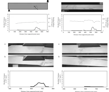
Distance from supported point (mm)
Residual Variance ( × 10 -4 mm 2) Bending Stiffness ( × 10 10 kN·mm 2 ) 0 1 2 3 4 5 6 7 8 0 1 1.5 2 2.5 3 700 600 500 400 300 200 100 Residual Variance ( × 10 -4 mm 2) Bending Stiffness ( × 10 10 kN·mm 2 )
Distance from supported point (mm)
0 1 2 3 4 5 6 7 8 1 1.5 2 2.5 3
0 100 200 300 400 500 600 700
Fig. 7. Profi les of bending
stiffness (broken line) and residual variance (solid line) from the FEM result (left) and from the bending test (right) (type 3 spike knot running from bottom left to top right,
local grain distortion causes the characteristic variations in the bending defl ection curve observed at the spike knots.
Images of typical failures that occurred during the destructive four-point bending test are illustrated in Fig. 9. The residual variance profi le over the loading span obtained from the polynomial regression curve of Eq. 4 is also shown below the images.
y PL
EI x Lx
L
= − ⎛ − +
⎝⎜
⎞ ⎠⎟
36 3 3 9
2
2
(4)
The specimens showing a clear peak in the residual variance profi le around the knots always ruptured at the knots (left side of Fig. 9), while the specimens without a clear peak did not always rupture at the knots (right side of Fig. 9). There-fore, we believe that the method employing the residual variance profi le of a bending defl ection curve can be used to distinguish between the two types of knots in the same manner as visual grading.
Conclusions
Bending defl ection curves across knots have been found to be characteristically distorted according to the types of knots. The residual variance between the measured defl ec-tion curve and the polynomial regression curve in regions with knots has been found to be higher than that of knot-free regions. Using a residual variance profi le, it is possible
to detect knots at which failures initiate. Comparison between the bending experiment and FEM analysis showed that cross-sectional reductions cause the characteristic vari-ations in the bending defl ection curve depending on the position of the encased knots. Local grain distortions also cause variations in the curve depending on the direction of spike knots.
In this study, bending tests were combined with an image analysis technique. The bending defl ection curves directly refl ected the mechanical properties of defects. Therefore, this method used in combination with machine stress grading may give a better estimation of strength-reducing effects of localized defects.
References
1. Mitsuhashi K, Poussa M, Puttonen J (2008) Method for predicting tension capacity of sawn timber considering slope of grain around knots. J Wood Sci 54:189–195
2. Iwasaki S, Sadoh T (1991) Measurements of knots in hinoki and sugi lumbers by the optical scanning method (in Japanese). Mokuzai Gakkaishi 37:999–1003
3. Sugimori M (1993) Recognition of longitudinal knot area by light refl ection and image processing (in Japanese). Mokuzai Gakkaishi 39:1–6
4. Pham DT, Alcock RJ (1998) Automated grading and defect detec-tion: a review. Forest Prod J 48:34–42
5. Estévez PA, Perez CA, Goles E (2003) Genetic input selection to a neural classifi er for defect classifi cation of radiata pine boards. Forest Prod J 53:87–94
Distance from supported point (mm)
Residual Variance
(
×
10
-4 mm 2)
Bending Stiffness
(
×
10
10
kN·mm
2
)
0 1 2 3 4 5 6 7 8
0 1
1.5 2 2.5 3
700 600 500 400 300 200 100
Residual Variance
(
×
10
-4 mm 2)
Bending Stiffness
(
×
10
10
kN·mm
2
)
0 1 2 3 4 5 6 7 8
1 1.5 2 2.5 3
Distance from supported point (mm)
0 100 200 300 400 500 600 700
Fig. 8. Profi les of bending
stiffness (broken line) and residual variance (solid line) from the FEM result (left) and from the bending test (right) (type 4 spike knot running from bottom right to top left,
P = 1.5 kN)
a
b
Distance from supported point (mm)
Residual Variance
(
×
10
-4
mm
2)
0 1 2 3 4 5 6 7 8
400 500 600 700 800
b a
Residual Variance
(
×
10
-4
mm
2)
0 1 2 3 4 5 6 7 8
Distance from supported point (mm)
400 500 600 700 800
Fig. 9a, b. Failure images and
profi le of residual variance
(P = 1.5 kN) a Lumber before
6. Boström L (1999) State of the art on machine strength grading. Proceedings of the 1st RILEM Symposium on Timber Engineer-ing, Stockholm, Sweden
7. Schajer GS (2001) Lumber strength grading using X-ray scanning. Forest Prod J 51:43–50
8. Sadoh T, Murata K (1993) Detection of knots in hinoki and kara-matsu lumber by thermography (in Japanese). Mokuzai Gakkaishi 39:13–18
9. Karsulovic JT, León LA, Gaete L (2000) Ultrasonic detection of knots and annual ring orientation in Pinus radiata lumber. Wood Fiber Sci 32:278–286
10. Baradit E, Aedo R, Correa J (2006) Knot detection in wood using microwaves. Wood Sci Technol 40:118–123
11. Schajer GS, Orhan FB (2006) Measurement of wood grain angle, moisture content and density using microwaves. Holz Roh Werkst 64:483–490
12. Murata K, Masuda M, Ukyo S (2005) Analysis of strain distribu-tion of wood using digital image correladistribu-tion method – four-point bend test of timber including knots (in Japanese). Trans Visualiz Soc Jpn 25:57–63
13. Forest Products Laboratory (1999) Wood handbook: wood as an engineering material. General Technical Report FPL-GTR-113, United States Department of Agriculture, Forest Service, Madison, WI, pp 4–14
14. Nagai H, Murata K, Nakamura M (2007) Defect detection of
lumber including knots using bending defl ection curve (in
Japanese). J Soc Mater Sci 56:326–331
15. Otsu N (1979) A threshold selection method from gray-level his-tograms. IEEE Trans Syst Man Cybern SMC-9:62–66
16. Cramer SM, Goodman JR (1983) Model for stress analysis and strength prediction of lumber. Wood Fiber Sci 15:338–349 17. Cramer SM, Goodman JR (1986) Failure modeling: a basis for
strength prediction of lumber. Wood Fiber Sci 18:446–459 18. Zandbergs JG, Smith FW (1988) Finite element fracture prediction
for wood with knots and cross grain. Wood Fiber Sci 20:97–106 19. Phillips GE, Bodig J, Goodman JR (1981) Flow-grain analogy.
Wood Fiber Sci 14:55–64
20. Mackenzie-Helnwein P, Eberhardsteiner J, Mang HA (2003) A multi-surface plasticity model for clear wood and its application to the fi nite element analysis of structural details. Comput Mech 31:204–218