R E S E A R C H
Open Access
Epidermis segmentation in skin
histopathological images based on thickness
measurement and k-means algorithm
Hongming Xu and Mrinal Mandal
*Abstract
Automatic segmentation of the epidermis area in skin histopathological images is an essential step for
computer-aided diagnosis of various skin cancers. This paper presents a robust technique for epidermis segmentation in the whole slide skin histopathological images. The proposed technique first performs a coarse epidermis
segmentation using global thresholding and shape analysis. The epidermis thickness is then measured by a series of line segments perpendicular to the main axis of the initially segmented epidermis mask. If the segmented epidermis mask has a thickness greater than a predefined threshold, the segmentation is assumed to be inaccurate. A second pass of fine segmentation using k-means algorithm is then carried out over these coarsely segmented result to enhance the performance. Experimental results on 64 different skin histopathological images show that the proposed technique provides a superior performance compared to the existing techniques.
Keywords: Histopathological image analysis, Epidermis segmentation, Epidermis thickness, Global threshold
Introduction
Skin cancer is among the most frequent and malignant types of cancer around the world [1]. Melanoma is the most aggressive type of skin cancer, which causes a large majority of skin cancer deaths. According to a recent statistics, about 76,690 people are diagnosed with skin melanoma, and about 9,480 died from it in the United States alone in 2013 [2]. The early detection and accurate prognosis of skin cancers will help to lower the mor-tality. However, the early diagnosis of skin cancers such as cutaneous melanoma is not trivial, as the malignant melanoma and benign tumors may have similar appear-ance in their early stages. Although many techniques have been developed for melanoma diagnosis, e.g., epilumi-nescence microscopy [1] and confocal microscopy [3], which can provide initial diagnosis, the histopathological examination of a whole slide image (WSI) by patholo-gists remains the gold standard for the diagnosis [4] as the histopathology slides provide a cellular level view of the disease [5].
*Correspondence: [email protected]
Department of Electrical and Computer Engineering, University of Alberta, T6G 2V4 Edmonton, Canada
Traditionally, the histopathological slides are examined under a microscope, and pathologists make the diagnosis based on their personal experience and knowledge. How-ever, the diagnosis by pathologists are typically subjective and often lead to intra- and inter-observer variability [6, 7]. For example, it has been reported that in the diagno-sis of melanoma, the inter-observer variation of diagnodiagno-sis sensitivity ranges from 55 to 100 % between 20 patholo-gists [8]. Besides, the manual analysis of the WSI with high resolution is labor intensive due to the large volume of the data to be analyzed [9]. To address these problems, computer-aided image analysis which can provide reliable and reproducible results is desirable.
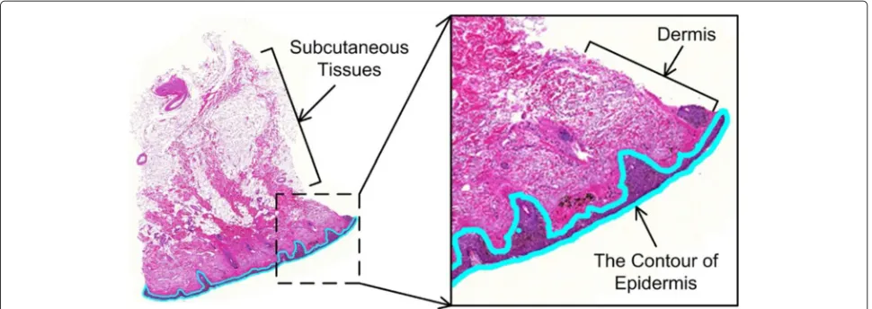
Figure 1 shows a skin WSI stained with hematoxylin and eosin (H&E). As observed in Fig. 1, a typical digitized skin slide can be divided into three main parts: epidermis, der-mis, and sebaceous areas. The automatic segmentation of epidermis area is an important step in melanoma diagno-sis by analyzing the histopathological images. The grading of the melanoma can generally be made by analyzing the architectural and morphological features of atypical cells in the epidermis or epidermis-dermis junctional area [10]. For example, the digitized skin slide shown in Fig. 1 is with superficial spreading melanoma, where the image looks
Fig. 1Example of skin tissue digital slide (superficial spreading melanoma). Note that the manuallylabeled contourof the epidermis area is superimposed on the WSI
like a normal skin tissue unless the epidermis area is exam-ined carefully. In addition, epidermis segmentation helps in identifying the relative positions between carcinoma cells and epidermis boundaries. The invasion depth of car-cinoma cells into the skin tissue can be measured, which is a critical indicator for skin caner grading and therapy [3].
Several works have been conducted for computer-aided diagnosis based on WSI. These works are related to neu-roblastoma [11, 12], cervical intraepithelial neoplasia [9], follicular lymphoma [13], and breast cancer [14]. In the automatic diagnosis of various cancers by analyzing dig-itized slides, the segmentation of histological structures (e.g., nuclei and glands) is significantly important [15]. Jung et al. [16] proposed a H-minima transform-based marker extraction method that segments cell nuclei in microscopic images by marked watershed algorithm. Lu et al. [17] proposed a technique that combines the prior knowledge (e.g., nuclei size and shape) and adaptive thresholding for nuclei segmentation in skin histopatho-logical images. Qi et al. [18] proposed to detect cell seeds in breast histopathological images by a single pass voting algorithm, and delineate cell contours by a repulsive level set model [19]. Sertel et al. [13] applied k-means clustering in theL∗a∗b∗ color space to segment nuclei, cytoplasm, and extracellular material which are used as features of follicular lymphoma grading. Zhang et al. [20] proposed an automated skin histopathological image annotation method which applies a graph-cutting algorithm to seg-ment skin image into disjoint regions and labels each region based on the correspondingly extracted features. Naik et al. [21] proposed a method of automatically detecting and segmenting glands in prostate histopatho-logical images. The technique first utilizes a Bayesian classifier based on low-level image features to detect the lumen, epithelial cell cytoplasm, and epithelial nuclei. The
detected lumen area is then used to initialize a level set curve, which is evolved to find the interior boundary of nuclei surrounding the gland structure. All of these tech-niques can potentially be used by skin image analysis and computer-aided system for melanoma diagnosis.
to remove all low-intensity components in the dermis area and keep the epidermis unchanged when dealing with the WSIs. Table 1 compares the related works on epidermis segmentation in skin histopathological images.
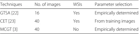
Since existing epidermis segmentation techniques are mainly based on global thresholding with area and shape analysis, they usually fail to provide a high precision when different dark skin components (e.g., cell nuclei, hair fol-licles) are present in the dermis area. Figure 2 compares segmentation results obtained by existing techniques with the manually labeled ground truth. Figure 2a shows a skin WSI with manually labeled epidermis contours in our database. Figure 2b–d shows the segmentation results by the GTSA [22], CET [23], and MCGT [3] techniques, respectively. It is observed in Fig. 2 that the existing tech-niques incorrectly segment many false positive regions in the dermis area as the epidermis area.
In this paper, we propose a new technique that over-comes the limitations of the existing techniques for epi-dermis segmentation in skin WSIs. The proposed tech-nique first performs a coarse epidermis segmentation on the WSI. The thickness of the coarsely segmented epi-dermis mask is then measured. The skin region corre-sponding to the epidermis mask that has a large thickness is analyzed again for a fine segmentation to improve the segmentation precision.
Materials and methods
In this section, we illustrate the image dateset used in this work and the proposed technique for epidermis segmen-tation.
Image dataset
The studied dataset was based on histopathological images from formalin-fixed paraffin-embedded tissue blocks of skin biopsies. The sections prepared are about 4 μmthick and are stained with H&E using an automated stainer. The skin tissue samples consist of 13 normal skins, 20 melanocytic nevi, and 31 skin melanomas. The original digital WSIs were captured under×40 magnifica-tion on Carl Zeiss MIRAX MIDI Scanning system. Since the original WSIs have a large volume size (each around 10 GB) and are difficult for real-time processing, these images were down-sampled by a factor of 32 (the same as the GTSA technique [22]) and saved into TIFF format using MIRAX Viewer software. Overall, the image dataset
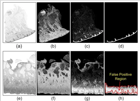
Table 1Related works on skin epidermis segmentation
Techniques No. of images WSIs Parameter selection
GTSA [22] 16 Yes Empirically determined
CET [23] 40 Yes From training images
MCGT [3] 40 No Empirically determined
consists of 64 different skin WSIs with the resolution between 2500×3000 and 6000×10,000 pixels.
Schematic of the proposed technique
The schematic of the proposed technique for epidermis segmentation is shown in Fig. 3. The technique has three modules. In the first module, the epidermis coarse seg-mentation is performed based on thresholding and shape analysis. In the second module, the thickness of coarsely segmented epidermis area is measured using line seg-ments perpendicular to the main axis of the epidermis mask. The coarsely segmented result is evaluated based on the measured epidermis thickness. In the third mod-ule, a second-pass fine segmentation by an unsupervised clustering algorithm is performed on the epidermis region with the poor quality segmentation result. The three mod-ules of the proposed technique are now presented in details in the following.
Coarse segmentation
Given an RGB imageIl, the red channelRlis selected for the epidermis coarse segmentation, since the red channel of the H&E stained skin histopathological image provides good distinguishable information [22]. With the red chan-nel imageRl, the epidermis coarse segmentation is then performed as follows:
(1) Removing white background pixels: In this step, we empirically select a thresholdτ1(e.g.,τ1 = 240) to
sepa-rate skin tissues from the background (which are typically white). The pixels inRlwith gray values smaller thanτ1are
classified as the foreground. Let the foreground pixels be denoted by{Fk}k=1...M, whereMis the number of pixels.
(2) Applying global thresholding: The Otsu’s threshold-ing technique [24] is applied to group the pixels{Fk}k=1...M into two classes. A binary maskb0is generated as follows:
b0
i,j=
1 if Fk≤τ2
0 if Fk> τ2 (1)
wherei,jis the 2D coordinate of the pixelFk inRl,τ2is
the threshold obtained by the Otsu’s technique.
(3) Eliminating false regions: We label all the regions in the binary maskb0via connected criterion. Let the
8-connected regions inb0be denoted by{Ck}k=1···Owhere Ois the number of connected regions. For each region Ck, we calculate the areaCarea, the major axis lengthrmaj,
and minor axis lengthrminof the best fit ellipse [25]. A
binary maskb1with epidermis regions as the foreground
is determined as follows:
b1(Ck)= ⎧ ⎨ ⎩
b0(Ck), if (Carea >Tarea)∧
rmajrmin>Tratio
0, otherwise
Fig. 2Comparison of automated epidermis segmentation and manually labeled ground truth.aA skin histopathological image with labeled epidermis contours.bGTSA technique [22].cCET technique [23].dMCGT technique [3]. Note that the segmentation results in (b–d) contain many false positive regions from the dermis
whereb0(Ck)represents the pixels of the regionCkinb0,
∧ is the AND operation, Tarea and Tratio are the
prede-fined thresholds. Note thatTareais used to remove small
noisy regions inb0, whileTratiois used to select the
epi-dermis region that has a long and narrow shape after global thresholding [22, 23]. In this work,TareaandTratio
values are determined based on the domain prior knowl-edge and experiments on training images. Specially, we set the thresholds as Tarea = 0.006M, andTratio = 3. For
more details, please refer to parameters selection in the “Performance evaluations” section.
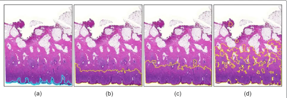
Figure 4 shows two examples of both intermediate and final coarse segmentation results. Figure 4d, h shows the segmented epidermis regions (b1) corresponding to
Fig. 4a, e, respectively. Note that Fig. 4d shows a good quality segmentation, whereas Fig. 4h shows a poor quality (incorrect) segmentation where the false positive region is highlighted by the manually labeled contour.
Thickness measurement
It is observed in Fig. 4 that coarse segmentation module may result in both good and poor quality segmentations. With a pixel resolution of 3.72μm/pixel, the segmented epidermis as shown in Fig. 4d on average has a thick-ness of 52 pixels (or 0.19 mm), whereas the segmented epidermis as shown in Fig. 4h has a thickness of 276 pix-els (or 1.03 mm). The epidermis varies in thickness in different regions of the body but should be within a lim-ited range [26]. In our database, the epidermis of skin histopathological images roughly has a thickness of 0.1– 0.4 mm, and hence a second-pass segmentation can be carried out based on thickness measurement. In this mod-ule, we measure the thickness of the coarsely segmented result to classify it as good or poor quality segmentation. The steps of thickness measurement are detailed below.
(1) Morphological preprocessing: In order to smooth the boundaries of the epidermis area, the morphological
Fig. 4Two examples of epidermis coarse segmentation.a,eRed channel images.b,fImages after removing background pixels.c,gBinary images after global thresholding.d,hFinal binary masks. Note thatwhite regionsin (d) and (h) correspond to segmented epidermis areas
closing operation is first performed on the mask b1 as
follows:
b2=b1•S (3)
where • is the morphological closing operator, andS is the structuring element. In this work, a disk-shaped struc-turing element with a radius of 10 pixels is empirically selected for the closing operation. Next, the holes within
the maskb2are filled by performing the morphological
reconstruction operation:
b3=
b2c,bm c
(4)
where is the morphological reconstruction opera-tor [27],bc2is the complement ofb2, andbmis the marker image which is set to be 0 everywhere except on the image border, where it is set to bebc2. Figure 5a shows a
maskb1[cropped from Fig. 4h], and Fig. 5b, c shows the
correspondingb2andb3.
(2) Thinning of epidermis mask: This step reduces the epidermis area in the maskb3to a connected stroke (a thin
line) that is only a single pixel wide. The connected stroke can be considered as the skeleton of the epidermis area. To obtain the connected stroke, the parallel thinning algo-rithm [28] is performed on the mask b3. The algorithm
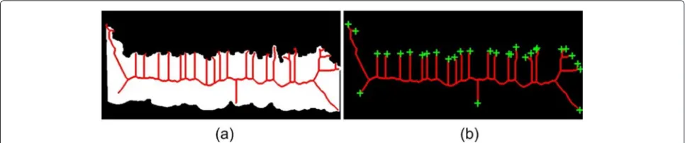
is executed in a number of iterations until the generated mask b4 stops changing. Figure 6a shows the generated
epidermis skeleton in the maskb4superimposed on the
maskb3.
(3) End point extraction: After generating the maskb4,
the end points of the epidermis skeleton are detected by a lookup table (LUT) technique [27]. A LUT is first con-structed based on the observation that an end point (in the epidermis skeleton) has exactly one foreground neighbor. The maskb4is then processed by using the generated LUT
to extract end points of the epidermis skeleton. Let the end points be denoted by{Ek}k=1...N, whereNis the number of end points. In Fig. 6b, the end points are marked with + symbols.
(4) Main axis identification: It is observed in Fig. 6a, b that there are many branches in the epidermis skeleton. The longest path joining two end points on the skeleton reflects the main axis of the maskb3. In this step, we
cal-culate all paths joining each possible pair of end points on the skeleton, and select the longest path as the main axis. Given two arbitrary end pointsEiandEj, let the geodesic distance (i.e., the number of pixels on the shortest path connectingEiandEj) be denoted byDij. The main axis is calculated as follows:
Step 1: Calculate all possibleDij based on the geodesic distance transform [29], where 1≤i,j≤N.
Step 2: Select the longest geodesic distance among all possibleDij and consider the corresponding constrained path as the main axis.
Step 3: Smooth the main axis by using a moving average filter of length 200 pixels.
Note that there is usually a large number of end points, and hence it may be computationally expensive to cal-culate all possible Dij in step 1. As observed in Fig. 6b, the pair of end points corresponding to the longest con-strained path usually has a relatively long Euclidean dis-tance. In order to speed up the main axis identification, we calculate the Euclidean distance between all possible end points, and select a short list of pairs (e.g., 10 pairs) based on (large) Euclidean distance. The main axis identification can then be efficiently performed by applying steps 1–3 on the selected pairs.
Let the obtained main axis be denoted by points set {Zk}k=1...QwhereQis the number of points on the main axis. Figure 7 illustrates the main axis identification with an example. Figure 7a shows a constrained path (the red line) joining pointsEiandEj. Figure 7b, c shows the epi-dermis main axis before smoothing and after smoothing, respectively, superimposed on the maskb3.
(5) Epidermis thickness calculation: In this step, we first calculate the gradient image of the mask b3, and select
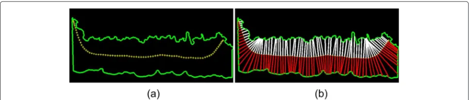
boundary positions with non-zero gradient magnitudes to obtain the epidermis boundary points set{Ak}k=1...W whereW is the number of points. We then calculate the epidermis thickness based on the epidermis main axis and epidermis boundary points. Note that there areQpoints on the main axis. In order to reduce the computational complexity, we calculate the epidermis thickness using selected points on the main axis. In this work, a set of r points, {Zk}k=h,2h,···,rh where r =
Q h
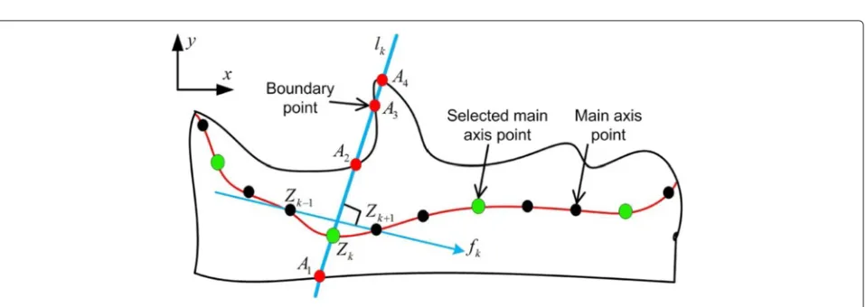
and h = 20, is selected. Figure 9a shows the epidermis contour with rselected points on the main axis. To calculate the epi-dermis thickness, a perpendicular line for each selected point on the main axis is defined. Given a pointZk(xk,yk) (see Fig. 8), the steps to calculate the local thickness are as follows.
Step 1: Letfk denote the directed line passing through pointsZk−1
xk−1,yk−1
andZk+1
xk+1,yk+1
. Note that the direction is from the pointZk−1toZk+1. The slopesk of the linelkperpendicular tofkis computed as follows:
Fig. 7Illustration of main axis identification.aA constrained path joiningEiandEj. Epidermis maskb3with the main axisbbefore smoothing andc after smoothing
sk= ⎧ ⎪ ⎪ ⎨ ⎪ ⎪ ⎩
0, ifxk+1=xk−1
∞, ifyk+1=yk−1
xk−1−xk+1
yk+1−yk−1, otherwise
(5)
Step 2: The intersection points between the line lk and the epidermis boundary {Ak}k=1...W are calculated. A boundary point Ak(uk,vk) is considered to be on the perpendicular linelkif it satisfies the following condition:
arctan(sk)−arctan
vk−yk uk−xk
≤η (6)
whereηis a small positive number (e.g.,η=0.05) to allow for a small error in intersection point calculation. Note that for an arbitrary pointZk there will be two or more intersection points. For example, in Fig. 8, the linelk inter-sects with the epidermis contour at four pointsA1,A2,A3,
andA4.
Step 3: The directed line fk divides the intersection points (e.g.,A1,A2,A3, andA4) into two groups: right side
points (RSP) and left side points (LSP). Note that RSP and LSP are seen from the direction of the linefk. The posi-tion of a point Ak(uk,vk) with respect to the line fk is determined by the following equation:
ϕ=ukα+vkβ+γ (7)
whereα=yk+1−yk−1,β=xk−1−xk+1,γ =xk+1yk−1−
xk−1yk+1. Ifϕ < 0, the point belongs to RSP (i.e.,Ak is located on the right side offk); ifϕ >0, the point belongs to LSP; ifϕ=0, the point is on thefk. In Fig. 8, the points A2,A3,A4are in the LSP, whereas the pointA1is in the
RSP.
Step 4: The local thicknesstkfor a pointZkis computed as follows:
tk =min
edisAi,Aj
, Ai∈RSP∧Aj∈LSP (8)
where edisAi,Aj
is the Euclidean distance between pointsAiandAj. In Fig. 8, the Euclidean distance between pointsA1andA2is computed as the local thicknesstk.
Likewise, the local thicknesses {tk}k=h,2h,···,rh for all selected points on the main axis are calculated by using steps 1–4. Figure 9b shows the line segments measuring epidermis thickness.
(6) Segmentation quality evaluation: The quality of coarse segmentation result is evaluated based on the aver-age value of measured epidermis thickness, which is as follows:
ρ=
1 if t< τ3
0 otherwise (9)
where ¯t = 1rrk=1tkh, τ3 is a threshold value and ρ is
a parameter to indicate the coarse segmentation quality.
Fig. 9Illustration of epidermis thickness measurement.aEpidermis contour with selected points on the main axis.bLine segments measuring epidermis thickness
Note that the thresholdτ3is determined based on
experi-ments on training images (please see parameters selection in the “Performance evaluations” section). In this work, we set the thresholdτ3as 150 pixels. For a good quality
segmentation,ρ =1, whereas for a poor quality segmen-tation, ρ = 0, which needs to be enhanced by the fine segmentation to be presented in the next module.
Fine segmentation
The coarse segmentation results are classified into good and poor quality segmentations based thickness mea-surement. In this module, we consider the poor quality segmentation for further analysis in order to obtain a more accurate segmentation.
When ρ = 0, it is likely that some dermis pixels are incorrectly classified as epidermis pixels. In order to obtain a more accurate segmentation, it is necessary to conduct a second-pass fine segmentation to divide the pixels into two classes (e.g., epidermis and dermis pix-els). To obtain a robust performance, we perform the second-pass fine segmentation by using {R,G,B} color channels. Due to the possible variations in the color spectrum between different digitized slides, k-means clas-sification [30], which is an unsupervised clasclas-sification algorithm, is selected to perform the fine segmentation. The{R,G,B}values of the pixels that are binary true in the coarsely segmented epidermis area (e.g., the maskb1) are
taken from the imageIland used as clustering attributes. The k-means algorithm divides the pixels into two classes
based on their attributes (e.g., {R,G,B} color values) by iteratively minimizing the following cost function:
J=
2
j=1
nj
i=1
xji−cj
2
(10)
where·is the Euclidean norm,njis the number of pixels in the classj,xjiis theith pixel in the classj, andcjis the centroid of the classj. Note that the number of classes is set as 2 that corresponds to dermis and epidermis.
Figure 10a shows the coarse segmentation result in Fig. 5a in color. Figure 10b, c shows two classes of pixels obtained by the k-means algorithm. It is observed that the class with epidermis pixels has relatively darker color (i.e., lower R,G,B values) than the class with dermis pixels. The two classes can be identified as follows:
k∗=
1 if R1+G1+B1
<R2+G2+B2
2 otherwise
(11)
whereR1,G1,B1
andR2,G2,B2
are the centroids of the two classes. Note that for the class with epidermis pixels, k∗=1, while for the class with dermis pixels,k∗=2;
The foreground pixels shown in Fig. 10c are consid-ered to be epidermis pixels according to the Equation 11. However, it is observed in Fig. 10c that a number of low-intensity pixels in the dermis area are classified as epidermis pixels. Note that most of the false positive
pixels (belonging to dermis area) are isolated pixels, or correspond to regions with smaller area. Therefore, false positive pixels can easily be eliminated by the area open-ing operation. Regions that have areas below the threshold Tarea (see the coarse segmentation module) are removed.
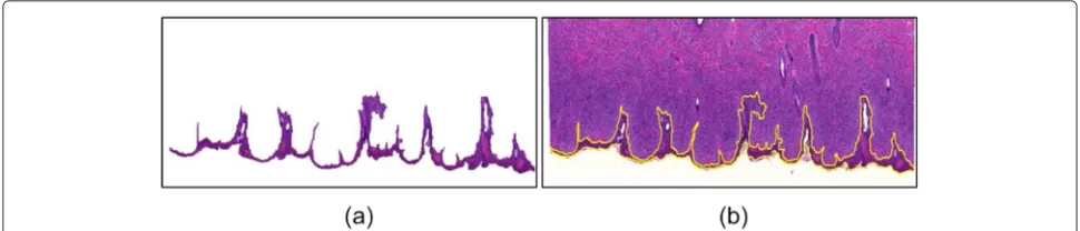
Finally, the morphological closing operation with a disk shape structuring element (with a radius of 5 pixels) is performed to smooth the epidermis area, and the holes within the epidermis area are filled by the reconstruction operation. Figure 11a shows the finally obtained epider-mis region. Figure 11b shows the epiderepider-mis contour on the original image.
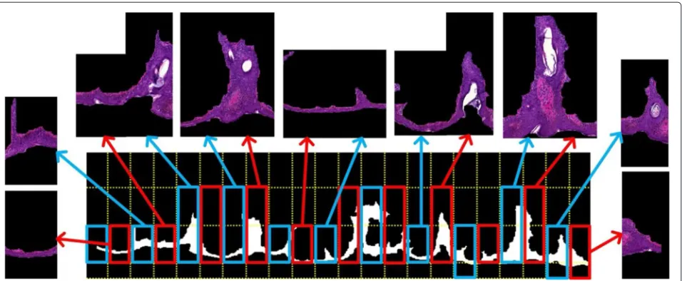
The segmented epidermis area can now be divided into several image tiles which are mapped to the high reso-lution field for further image analysis [22]. For example, the high-resolution image tiles can be further processed for nuclei segmentation [5, 17] and melanocytes detec-tion [31]. The features extracted from the epidermis area provide important indicators for computer-aided skin melanoma diagnosis. The details of image tiles genera-tion can be found in [22]. Figure 12 shows an example of generated high-resolution image tiles.
Performance evaluations
In this section, we illustrate the comparative epidermis segmentation results by the proposed technique and exist-ing techniques.
Evaluation metrics
The automatic epidermis segmentation results are com-pared to the ground truth segmentation results obtained by visual inspection. The evaluations are performed by computing area based metrics [22] namely preci-sion (APRE), sensitivity (ASEN), and specificity (ASPE),
and boundary based metrics [32] namely Hausdorff distance (DHD) and mean absolute distance (DMAD). We denote the manually obtained boundary as g =
cgi|i∈(1, 2,· · ·,m), and the boundary of the automatic
segmentation ass =
csjj∈(1, 2,· · ·,n)
, wheremand nare the numbers of the ground truth and automatically
segmented boundary points, respectively. The area based metrics are defined as follows:
APRE=
(s)∩ g
| (s)| ×100 % (12)
ASEN=
(s)∩ g
g ×100 % (13)
ASPE=
(s)∩ g
g ×
100 % (14)
where (·)is the area of the closed boundary,|·|is the car-dinality operator,∩is the intersection operation and (·) is the complement of (·). To evaluate the automatically segmented boundary contours, we calculate the distance of every point ingfrom all points ins. The boundary based metrics are defined as follows:
DHD=max
i
min j
csj−cgi
(15)
DMAD=
1 m
m
i=1
min j
csj−cgi
(16)
where · is the 2D Euclidean distance between two points. The Hausdorff distance (DHD) measures the worst
possible disagreement between two contours. The mean absolute distance (DMAD) estimates the disagreement
averaged over the two contours.
Parameters selection
There are 64 different skin histopathological images in the whole dataset, which are provided with ground truth seg-mentations obtained manually. The 64 WSIs consist of three categories: 13 normal skins, 20 melanocytic nevi, and 31 skin melanomas. Note that there are three param-eters that should be selected appropriately in the pro-posed technique, which includesTarea,Tratio(thresholds
for eliminating false positive regions), and τ3
(thresh-old to determine the coarse segmentation quality). To determine the values of these parameters, we randomly selected 4 normal skins, 6 melanocytic nevi, and 8 skin melanomas as training images, which were used during
Fig. 12Example of generated image tiles. Note thatrectanglesmark the interested image tiles for further processing. Somesnapshotsof image tiles are present
the development of the technique. The 18 training images were randomly selected from each category to avoid any bias. The other 46 images were taken as testing images, which were used as an independent validation set. The values of training parameters are shown in Table 2. We explain the process of determining parameters’ values in the following.
To determine an adaptive threshold value forTarea, we
calculate the portion of epidermis pixels about skin tissue pixels in training images. It has been found that the por-tion of epidermis pixels ranged between 0.007 and 0.06, and hence the thresholdTarea is set as 0.006MwhereM
is the number of foreground pixels (i.e., skin tissue pixels) in the WSI. Similarly, we calculate the ratiormaj
rminfor
all ground truth epidermis regions in training images, and the rmaj
rmin values have been found to be in the range
between 3.3 and 26.6. Therefore, the thresholdTratiois set
as 3.
The parameterτ3is determined based on experiments
on training images in this work. Based on visual exami-nation, the coarsely segmented result of training images are divided into two groups: subsets A and B. In subset A (11 WSIs), the segmented results are quite similar to the ground truths, while in subset B (7 WSIs) a large num-ber of false positive pixels in dermis area are classified as epidermis pixels. The coarsely segmented masks of subset
Table 2Training parameters in the proposed technique
Modules Parameters Values
Coarse segmentation Tarea 0.006Mpixels
Coarse segmentation Tratio 3
Thickness measurement τ3 150 pixels
B have markedly large thickness than masks of subset A. Table 3 shows the performance evaluations of subsets A, B by the area-based metrics, and the corresponding aver-age epidermis mask thicknessx. As observed in Table 3, the segmentation precision for the subset B is significantly low, only 38.69 %. The average thickness xfor subset B is 211.60 pixels, which is much higher than 63.26 pixels for subset A. The boxplot for the epidermis thickness of subsets A and B is shown in Fig. 13. Based on the results observed in Fig. 13, the thresholdτ3is finally set as 150
pixels.
In order to test how sensitivities are the parameters’ val-ues to the choice of training images, we selected another set of 18 skin images randomly (from the testing images) and calculated the values of Tratio, Tarea, and τ3
follow-ing a similar process of parameter selection. Experiments show that the values of these three parameters only have marginal variations (Tratio = 0.007M, Tarea = 3 and τ3= 155). In other words, the parameters’ values do not
fluctuate too much across databases.
Quantitative results
To illustrate the efficacy of the proposed epidermis seg-mentation technique, the performance of the proposed technique is compared with the existing epidermis seg-mentation techniques including the GTSA [22], CET [23],
Table 3Performance evaluations of epidermis coarse segmentation in subsets of training images
Subsets APRE(%) ASEN(%) ASPE(%) x(pixels)
A 98.11 97.04 99.96 63.26
Fig. 13Thickness variations of coarsely segmented epidermis masks in subsets A and B of training images. Subset A (B) includes images with correct (incorrect) segmentations after coarse segmentation module
and MCGT [3] techniques. The GTSA technique has two parametersTareaandTratio, which were set the same
val-ues as our proposed technique. The CET technique has several key parameters including the low output thresh-olds for contrast enhancement, the sizes of smoothing mean filter and morphological operations and the thresh-olds to eliminate noisy regions after thresholding. For the parameters (e.g., the size of smoothing filter) that are not used in the proposed technique, we set them following the work in [23]. While for parameters (e.g., Tarea used
to eliminate noisy regions) that are used in the proposed technique, we set them the same values as our proposed technique. The MCGT technique has only one key param-eter that is the size the structuring element for closing operation. To determine an optimal size for structuring element, we selected a set of values from 20 to 50 with a step of 5 to do experiments. 30 is finally determined as the size of the structuring element, as it provides the best performance of epidermis segmentation in our training images.
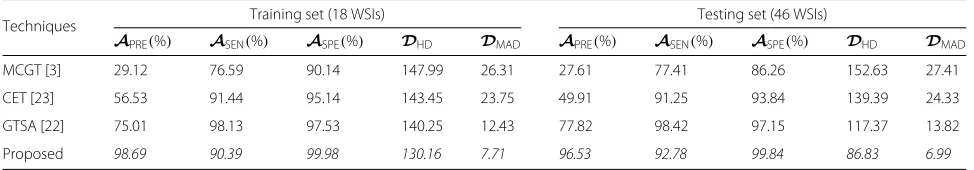
The average results of quantitative evaluations by Equations 12–16 on both training and testing sets are shown in Table 4. It is observed in Table 4 that the
proposed technique provides an overall superior per-formance in epidermis segmentation than the existing techniques. Although the sensitivities of the proposed technique (90.39 and 92.78 %) are marginally lower than those of the GTSA [22] technique, the proposed technique achieves much higher precisions (98.69 and 96.53 %), roughly 20 % higher than the GTSA technique. k-means algorithm used by fine segmentation module of the pro-posed technique incorrectly classifies a small number of epidermis pixels as dermis pixels, which results in the marginal drop in sensitivity. The poor performances of the GTSA and CET techniques are mainly because a large number of dermis pixels are incorrectly classified as epi-dermis pixels in images where there are a large number of cell nuclei in the dermis area. The cell nuclei in the dermis area appear dark purple, and global thresholding incorrectly considers them as epidermis pixels. In addi-tion, the CET technique [23] applies global thresholding on an equally weighted linear combination of the grayscale (Y channel) andb∗channel (e.g.,b∗inL∗a∗b∗color space) images, which provides a poor performance than using the red channel in our database. The performance of the MCGT [3] technique is much poorer than that of the other techniques, as it does not work on skin WSIs which include epidermis, dermis, and sebaceous areas. The MCGT technique assumes that the closing opera-tion can remove all unrelated components (typically dark appearance) in the skin dermis area, and hence the epider-mis area can be segmented out by thresholding. However, the dermis areas of WSIs contain many different dark skin components such as hair follicles, sweat glands, and nuclei clumps. Since the size of different skin components may vary greatly, it is difficult to define an appropriate struc-turing element for closing operation which can remove all unrelated skin tissues and keep the epidermis area unchanged. It is also noted from the Table 4 that the proposed technique has achieved relatively smallerDHD
andDMAD values in both training and testing sets, and hence the proposed technique provides a better matching between the ground truth contours and the automatically segmented contours.
For further comparison of the proposed technique with existing techniques, the thickness of automatically
Table 4Quantitative evaluations of epidermis segmentation between existing techniques and proposed technique
Techniques Training set (18 WSIs) Testing set (46 WSIs)
APRE(%) ASEN(%) ASPE(%) DHD DMAD APRE(%) ASEN(%) ASPE(%) DHD DMAD
MCGT [3] 29.12 76.59 90.14 147.99 26.31 27.61 77.41 86.26 152.63 27.41
CET [23] 56.53 91.44 95.14 143.45 23.75 49.91 91.25 93.84 139.39 24.33
GTSA [22] 75.01 98.13 97.53 140.25 12.43 77.82 98.42 97.15 117.37 13.82
Fig. 14Comparison of epidermis thickness between manually labeled epidermis masks and automatically obtained results for testing images. Note that the thickness of epidermis mask obtained by the proposed technique is very close to that of the ground truth, whereas the MCGT [3], CET [23], and GTSA [22] techniques tend to provide much larger thickness than the manually labeled ground truth
segmented epidermis masks of different techniques was measured by the proposed thickness measurement method (see thickness measurement module), and com-pared with the thickness of manually labeled epider-mis masks. Figure 14 shows the thickness comparisons between the automatically segmented masks and ground truth masks for 46 testing images. It is observed in Fig. 14 that the thickness of epidermis mask obtained by the pro-posed technique is very close to that of manually labeled epidermis mask, whereas the segmented epidermis masks by existing techniques tend to have much larger thickness than manually labeled epidermis masks. The MCGT [3], CET [23], and GTSA [22] techniques incorrectly segment some low-intensity areas (e.g., cell nuclei) in the dermis area as the epidermis area, which increases the thickness of the segmented epidermis mask.
Qualitative results
Qualitative results of epidermis segmentation for a whole slide skin histopathological image is illustrated in Fig. 15. Note that Fig. 15a shows the WSI with the manually labeled epidermis contour, while Fig. 15d, g, j, m shows the corresponding automatically segmented results by the MCGT [3], CET [23], GTSA [22], and the proposed tech-nique, respectively. Figure 15b, c, e, f, h, i, k, l, n, o shows the corresponding selected parts of magnified segmenta-tion results. Note that the magnificasegmenta-tion of selected parts are indicated by the rectangles on the WSIs. It is observed in Fig. 15 that the proposed technique provides more accurate segmentations than existing epidermis segmen-tation techniques. The MCGT [3] technique segments many false positive regions in the dermis area as the epi-dermis area, as a simple closing operation fails to remove
dark regions in the dermis area which are subsequently classified as the epidermis area by thresholding. The CET [23] and GTSA [22] techniques incorrectly segment many low intensity dermis areas as epidermis areas, since these low-intensity areas are segmented as binary fore-grounds by thesholding but not eliminated by subsequent shape and area analysis.
Computational complexity
All experiments were done on a 1.80 GHz Intel Core II Duo CPU, with 16 GB of RAM memory using MAT-LAB version R2013a. The proposed technique roughly takes 4.2 s to perform the epidermis segmentation for a whole slide skin histopathological image with size of 3200 × 3000 pixels, while the MCGT [3], CET [23], and GTSA [22] technique, respectively, take about 1.5, 3.3, and 0.9 s to process the same skin histopathological image.
Conclusions
Fig. 15Comparative segmentation results on a skin WSI.aManually labeled epidermis contour.b,cMagnification of selected parts in (a).d MCGT [3].e,fMagnification of selected parts in (d).gCET [23].h,iMagnification of selected parts in (g).jGTSA [22].k,lMagnification of selected parts in (j).mProposed technique.n,oMagnification of selected parts in (m). Note that a large number of dermis pixels are incorrectly segmented as epidermis pixels in (d,g,j). Distance annotations with a pixel resolution of 3.72μm/pixel are added on (a–c)
using the k-means algorithm is performed. The eval-uation on 64 different skin histopathological images shows that the proposed technique provides a superior performance than the existing techniques in epidermis segmentation.
Competing interests
The authors declare that they have no competing interests.
Acknowledgements
The authors would like to thank Dr. Naresh Jha, and Dr. Muhammad Mahmood of the University of Alberta Hospital for providing the images. We also would like to thank Dr. Cheng Lu of Shaaxi Normal University for providing the code of the GTSA technique.
Received: 5 December 2014 Accepted: 10 June 2015
References
1. I Maglogiannis, CN Doukas, Overview of advanced computer vision systems for skin lesions characterization. IEEE Trans. Inf. Technol. Biomed. 13(5), 721–733 (2009)
2. R Siegel, D Naishadham, A Jemal, Cancer statistics, 2013. CA Cancer J. Clin. 63(1), 11–30 (2013)
3. M Mokhtari, M Rezaeian, S Gharibzadeh, V Malekian, Computer aided measurement of melanoma depth of invasion in microscopic images. Micron.61, 40–48 (2014)
5. H Xu, C Lu, M Mandal, An efficient technique for nuclei segmentation based on ellipse descriptor analysis and improved seed detection algorithm. IEEE J. Biomed. Health Inf.18(5), 1729–1741 (2013) 6. SM Ismail, AB Colclough, JS Dinnen, D Eakins, D Evans, E Gradwell, JP
O’Sullivan, JM Summerell, RG Newcombe, Observer variation in histopathological diagnosis and grading of cervical intraepithelial neoplasia. BMJ: Br. Med. J.298(6675), 707 (1989)
7. S Petushi, FU Garcia, MM Haber, C Katsinis, A Tozeren, Large-scale computations on histology images reveal grade-differentiating parameters for breast cancer. BMC Med. Imaging.6(1), 14 (2006) 8. L Brochez, E Verhaeghe, E Grosshans, E Haneke, G Piérard, D Ruiter, J-M
Naeyaert, Inter-observer variation in the histopathological diagnosis of clinically suspicious pigmented skin lesions. J. Pathol.196(4), 459–466 (2002)
9. Y Wang, D Crookes, OS Eldin, S Wang, P Hamilton, J Diamond, Assisted diagnosis of cervical intraepithelial neoplasia (cin). IEEE J. Selected Topics Signal Process.3(1), 112–121 (2009)
10. G Massi, PE LeBoit,Histological Diagnosis of Nevi and Melanoma, 2nd edn. (Springer, Berlin, 2013)
11. O Sertel, J Kong, H Shimada, U Catalyurek, JH Saltz, MN Gurcan, Computer-aided prognosis of neuroblastoma on whole-slide images: Classification of stromal development. Pattern Recognit.42(6), 1093–1103 (2009) 12. J Kong, O Sertel, H Shimada, KL Boyer, JH Saltz, MN Gurcan,
Computer-aided evaluation of neuroblastoma on whole-slide histology images: classifying grade of neuroblastic differentiation. Pattern Recognit. 42(6), 1080–1092 (2009)
13. O Sertel, J Kong, UV Catalyurek, G Lozanski, JH Saltz, MN Gurcan, Histopathological image analysis using model-based intermediate representations and color texture: follicular lymphoma grading. J. Signal Process. Syst.55(1-3), 169–183 (2009)
14. V Roullier, O Lézoray, V-T Ta, A Elmoataz, Multi-resolution graph-based analysis of histopathological whole slide images: application to mitotic cell extraction and visualization. Comput. Med. Imaging Graph.35(7), 603–615 (2011)
15. MN Gurcan, LE Boucheron, A Can, A Madabhushi, NM Rajpoot, B Yener, Histopathological image analysis: a review. IEEE Rev. Biomed. Eng.2, 147–171 (2009)
16. C Jung, C Kim, Segmenting clustered nuclei using h-minima transform-based marker extraction and contour parameterization. IEEE Trans. Biomed. Eng.57(10), 2600–2604 (2010)
17. C Lu, M Mahmood, N Jha, M Mandal, A robust automatic nuclei segmentation technique for quantitative histopathological image analysis. Anal. Quant. Cytol. Histol.34, 296–308 (2012)
18. X Qi, F Xing, DJ Foran, L Yang, Robust segmentation of overlapping cells in histopathology specimens using parallel seed detection and repulsive level set. IEEE Trans. Biomed. Eng.59(3), 754–765 (2012)
19. P Yan, X Zhou, M Shah, ST Wong, Automatic segmentation of high-throughput RNAI fluorescent cellular images. IEEE Trans. Inf. Technol. Biomed.12(1), 109–117 (2008)
20. G Zhang, J Yin, Z Li, X Su, G Li, H Zhang, Automated skin biopsy histopathological image annotation using multi-instance representation and learning. BMC Med. Genomics.6(Suppl 3), 10 (2013)
21. S Naik, S Doyle, M Feldman, J Tomaszewski, A Madabhushi, inProceedings of the Second International Workshop on Microscopic Image Analysis with
Applications in Biology. Gland segmentation and computerized Gleason
grading of prostate histology by integrating low-, high-level and domain specific information (MIAAB, Piscataway NJ, USA, 2007), pp. 1–8 22. C Lu, M Mandal, inProceeding of the 2012 Annual International Conference
of the IEEE Engineering in Medicine and Biology Society. Automated
segmentation and analysis of the epidermis area in skin histopathological images (EMBC San Diego, CA, USA, 2012), pp. 5355–5359
23. JM Haggerty, XN Wang, A Dickinson, J Chris, EB Martin,et al, Segmentation of epidermal tissue with histopathological damage in images of haematoxylin and eosin stained human skin. BMC Med. Imaging.14(1), 7 (2014)
24. N Otsu, A threshold selection method from gray-level histograms. IEEE Trans. Syst. Man Cybern.11(285-296), 23–27 (1975)
25. A Fitzgibbon, M Pilu, RB Fisher, Direct least square fitting of ellipses. IEEE Trans. Pattern Anal. Mach. Intell.21(5), 476–480 (1999)
26. S Kusuma, RK Vuthoori, M Piliang, JE Zins, inPlastic and Reconstructive
Surgery. Skin anatomy and physiology (Springer London, 2010),
pp. 161–171
27. R Gonzalez, R Woods,Digital Image Processing, 3rd edn. (Prentice Hall, USA, 2008)
28. Z Guo, RW Hall, Parallel thinning with two-subiteration algorithms. Commun. ACM.32(3), 359–373 (1989)
29. P Soille,Morphological Image Analysis: Principles and Applications. (Springer, New York, 2003)
30. J MacQueen, inProceedings of the Fifth Berkeley Symposium on
Mathematical Statistics and Probability. Some methods for classification
and analysis of multivariate observations (Oakland, CA, USA, 1967), pp. 281–297
31. C Lu, M Mahmood, N Jha, M Mandal, Detection of melanocytes in skin histopathological images using radial line scanning. Pattern Recognit. 46(2), 509–518 (2013)
32. H Fatakdawala, J Xu, A Basavanhally, G Bhanot, S Ganesan, M Feldman, JE Tomaszewski, A Madabhushi, Expectation–maximization-driven geodesic active contour with overlap resolution (emagacor): Application to lymphocyte segmentation on breast cancer histopathology. IEEE Trans. Biomed. Eng.57(7), 1676–1689 (2010)
Submit your manuscript to a
journal and benefi t from:
7Convenient online submission 7Rigorous peer review
7Immediate publication on acceptance 7Open access: articles freely available online 7High visibility within the fi eld
7Retaining the copyright to your article