RVSIM: a feature similarity method for full-reference image quality assessment

(1)

R E S E A R C H

Open Access

RVSIM: a feature similarity method for

full-reference image quality assessment

Guangyi Yang

*

, Deshi Li, Fan Lu, Yue Liao and Wen Yang

Abstract

Image quality assessment is an important topic in the field of digital image processing. In this study, a full-reference image quality assessment method called Riesz transform and Visual contrast sensitivity-based feature SIMilarity index (RVSIM) is proposed. More precisely, a Log-Gabor filter is first used to decompose reference and distorted images, and Riesz transform is performed on the decomposed images on the basis of monogenic signal theory. Then, the

monogenic signal similarity matrix is obtained by calculating the similarity of the local amplitude/phase/direction characteristics of monogenic signal. Next, we weight the summation of these characteristics with visual contrast sensitivity. Since the first-order Riesz transform cannot clearly express the corners and intersection points in the image, we calculate the gradient magnitude similarity between the reference and distorted images as a feature, which is combined with monogenic signal similarity to obtain a local quality map. Finally, we conduct the monogenic phase congruency using the Riesz transform feature matrix from the reference image and utilize it as a weighted function to derive the similarity index. Extensive experiments on five benchmark IQA databases, namely, LIVE, CSIQ, TID2008, TID2013, and Waterloo Exploration, indicate that RVSIM is a robust IQA method.

Keywords: Image quality assessment, Riesz transform, Log-Gabor filter, Gradient magnitude, Visual contrast sensitivity

1 Introduction

Digital image is an essential factor to express and com-municate information. Digital imaging has been applied in many fields, but digital image quality is inevitably reduced and affected during image collection, compression [1–3], transmission [4], processing [5], and reconstruction [6,7]. The accurate assessment of image quality has also become challenging [8]. As such, image quality assessment (IQA) has been extensively investigated [9–11].

IQA can be divided into full-reference (FR), reduced-reference (RR), and no-reduced-reference (NR) assessments [12] based on the presence of reference images. The FR IQA methods are based on “the original image” , which is taken as the reference image. It is mainly used in assessing the similarity and fidelity between distorted image and origi-nal undistorted image [13,14]. The RR IQA methods are considered practical when we can only get access to some extracted features instead of the whole original image [15]. We can use these provided features and give a reasonable estimation on the distorted image’s quality [16]. In some

*Correspondence:ygy@whu.edu.cn

School of Electronic Information, Wuhan University, 430072 Wuhan, China

practical applications, the reference image is not available to perform a comparison against. Therefore, the NR IQA methods are needed [17]. This study focuses on FR IQA methods.

MSE and PSNR are widely used FR IQA methods. In these methods, image quality is assessed by calculating the overall pixel error, and average error is used as the final assessment result. These methods provide several advan-tages, such as simple calculation and easy implementation. But since the modeling is too simple, the comprehend-ing of the image is overly superficial. The absolute error between pixels of two images is calculated, but the corre-lation between pixels and the perceptive characteristics of human visual system (HVS) are disregarded. Their low-level features, such as edge information, are also yet to be described. Thus, it causes serious incongruency, which is against the perceptive characteristics of HVS and is likely the cause of unrealistic conditions between assessed results and actual phenomena during quality assessment [18,19].

Many representative assessment methods have been proposed to adapt to human visual characteristics. Wang et al. [12] established a Structural SIMilarity (SSIM)

International License (http://creativecommons.org/licenses/by/4.0/), which permits unrestricted use, distribution, and

(2)

model, which is considered the most common repre-sentative based on universal image quality index (UQI) [20]. The structural information of images is applied to assess quality and SSIM index. Experiments show that SSIM is appropriate than previous assessment methods. Although SSIM improves the congruency between assess-ment results and HVS perception, the structural features of images remain scalar and consequently causes SSIM to lose its validity when images are highly blurred. Numer-ous methods, such as MS-SSIM [21], ESSIM [22], GSSIM [23], 3-SSIM [24], CW-SSIM [25], and IW-SSIM [26], have been improved on the basis of SSIM, and these methods enhance the assessment result to a certain level. Sheikh et al. [27,28] also developed methods, such as IFC and VIF, based on natural scene statistics (NSS) to introduce the concept of information fidelity. Zhang et al. [29] pro-posed a Feature SIMilarity (FSIM) method that introduces phase congruency (PC) and gradient magnitude (GM) similarity as assessment features.

With in-depth research, natural images as a two-dimensional signal characterized by highly structured fea-tures must have a vector trait. The pixels of images show a strong dependency, which constitutes the structure of two-dimensional image. The main function of HVS is to obtain structural information from the field of view. Zhang et al. [30] constructed similarity matrices by using the characteristic map of first- and second-order Riesz transforms and utilized edge features as pooling func-tion to derive the RFSIM index because of the good performance of Riesz transform in multidimensional sig-nal processing. Luo et al. [31] introduced monogenic phase congruency (MPC) based on PC and proposed the RMFSIM method. With these methods, the structural method can be used to assess the vector characteristics of two-dimensional images more efficiently. However, these methods simply apply the Riesz transform to construct local features that partially consider the physical meaning of monogenic signal (MS) theory. Moreover, these assess-ment factors describe high-frequency information, such as edge features. The complexity of HVS has not yet to be fully presented. Hence, there is still much room for improvement.

In this study, a FR IQA method called Riesz transform and Visual contrast sensitivity-based feature SIMilarity index (RVSIM) is proposed by combining Riesz trans-form with visual contrast sensitivity. To the best of our knowledge, the Log-Gabor filter and the contrast sensitiv-ity function (CSF) are all well-known theories. However, we are the first to combine the frequency characteristic of Log-Gabor filter and frequency-sensitive features of HVS, so that the objective and subjective evaluation results are consistent as much as possible. In addition, although Riesz transform in multidimensional signal processing performs well, the first-order Riesz transform cannot clearly express

the corners and intersection points in the image. The proposed RVSIM method introduces the GM similarity thus improves the assessment of performance. In gen-eral, RVSIM takes full advantage of the MS theory [32] and Log-Gabor filter [33] by exploiting visual CSF [34] to allocate the weights of different frequency bands. The similarity matrix is obtained by introducing GM, and the MPC map is utilized as a pooling function to derive the final IQA score. Two groups of simulated experiments were carried out with two kinds of databases. The one kind is the LIVE, CSIQ, TID2008, and TID2013 databases, which mainly assess performance through calculating the absolute indicators of the method. The other kind is the Waterloo Exploration database, which mainly assesses through calculating the competitive ranking among meth-ods. The experimental results demonstrate that the pro-posed RVSIM method is a robust IQA method.

Notably, RVSIM is different from RFSIM [30] and RMF-SIM [31] in four aspects. First, RVSIM employs Log-Gabor band-pass filters on the reference and distorted images to obtain the components of images in differ-ent frequency bands. Second, RVSIM does not directly use the Riesz transform to determine the feature matrix. Instead, RVSIM utilizes the analytic space obtained by Riesz transform, including local amplitude, phase, and direction, which constitute a complete orthogonal basis [35], and subsequently calculates local feature similar-ities. Third, RVSIM applies the characteristics of HVS to assign different weights to various frequency bands. In this manner, the RVSIM model has appropriate con-gruency with the perceptive characteristics of the HVS. Fourth, RVSIM introduces the GM similarity and demon-strates that the first-order Riesz transform cannot clearly express the corners and intersection points in images.

The remaining parts of this paper are organized as fol-lows: Section2presents the MS theory, Log-Gabor filter, MPC, and visual contrast sensitivity. For the specific appli-cation of these theories in this study, we give a detailed design ideas and calculation process. Section3introduces the structure of the new IQA method proposed in this study and also describes the combination of MS, CSF, GM, and MPC to derive the RVSIM index. Section4presents the experimental results. Section5draws the conclusion.

2 Related works

2.1 Riesz transform

(3)

high-dimensional Euclidean space, which is suitable for image processing applications [38,39].

Figure1shows that the Riesz transform space is a spher-ical coordinate system in a 3D Euclidean space.R,R1, and R2are the projections of the points in the spherical coordi-nate system on the three axes [40]. In this spatial domain, the local amplitudeA, the local directionθ, and the local phaseϕcan be expressed as:

⎧ ⎪ ⎪ ⎨ ⎪ ⎪ ⎩

AR(x,y) =R(x,y)2₊_R₁₍_x_,_y₎2₊_R₂₍_x_,_y₎2

θR(x,y) =tan−1(−R2(x,y)/R1(x,y))

ϕR(x,y) =tan−1(R12(x,y)/R(x,y))

(1)

whereR12(x,y)=

R1(x,y)2+R2(x,y)2,θR(x,y)∈[ 0,π),

ϕR(x,y)∈[ 0,π).

2.2 Log-Gabor filter

Given that the length of the image signal is limited, the image signal is usually band-pass filtered before the Riesz transform, usually using the Log-Gabor filter [41]. In prac-tical applications, multiple Log-Gabor filters should be used to build a complete filter bank in the radial and hor-izontal directions because of the bandwidth limitation of a single Log-Gabor filter [42]. The optimum filter bank for a specific application can be established on the basis of previously described methods [43, 44]. In this study, the number of scalesnr = 5, the number of orientations nθ =1, and the splicing parameters are discussed in detail in Section4.1.

Section 2.4 shows that the center frequencies

ω0i(i=1,. . ., 5)of the filter bank areω01= 1₃,ω02= ₃12.1,

Fig. 1The Riesz transform space

ω03 = ₃2.11×2.1,ω04 = ₃2.11×2.1, and ω05 = ₃2.1×2.11×2.1×2.1. The bands of the Log-Gabor filter bank are [0.4786, 0.2026], [0.2611, 0.0965], [0.1243, 0.0460], [0.0591, 0.0221], and [0.0282, 0.0105]. Using this filter bank, the image R is filtered to complete the five-scale decom-position of the image, and the decomposed images Rbi(i = 1,. . ., 5)are obtained. The MS of the reference image

Rbi,Rbi₁,Rbi₂

(i = 1,. . ., 5) are obtained using Rbi (i = 1,. . ., 5)for the Riesz transform. Thus, Eq. (1) becomes:

⎧ ⎪ ⎪ ⎪ ⎪ ⎨ ⎪ ⎪ ⎪ ⎪ ⎩

Abi_R(x,y) = Rbi₍_x_,_y₎2₊_Rbi

1(x,y)2+Rbi2(x,y)2

θbi

R(x,y) =tan−1

−Rbi₂(x,y)/Rbi₁(x,y)

ϕbi

R(x,y) =tan−1

Rbi₁₂(x,y)/Rbi₍_x_,_y₎

(2)

where Rbi₁₂(x,y) = Rbi₁(x,y)2₊_Rbi

2(x,y)2,θRbi(x,y) ∈

[ 0,π),ϕ_Rbi(x,y) ∈[ 0,π),i = 1,. . ., 5. Similarly, the MS of the distorted image isDbi,Dbi₁,Dbi₂(i=1,. . ., 5)and the

corresponding local amplitudeAbi_D, the local directionθ_Dbi, and the local phaseϕ_Dbi,i=1,. . ., 5.

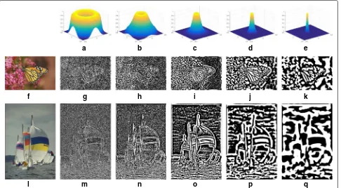
In this study, the Log-Gabor filter bank is shown in Fig. 2. The center frequencies ω0i (i = 1,. . ., 5) from

Fig.2a–eareω01 = 1₃,ω02 = ₃12.1,ω03 = ₃2.11×2.1,ω04 = 1

32.1×2.1×2.1, andω05 = ₃2.1×2.11×2.1×2.1. Using this Log-Gabor filter bank, two sample images (which aremonarchand sailing2 in the LIVE database [45]) are filtered to obtain the different components of the corresponding five bands. Notably, the sample images are grayed before filtering.

Figure2also shows that the Log-Gabor filter whoseω0 is set as1₃ reflects the high-frequency components of the image, mainly representing the most detailed information of the original image. The Log-Gabor filter, whoseω0is set as ₃1_2.1, reflects the sub-high frequency components of the image. The Log-Gabor filter whose ω0 is set as

1

32.1×2.1×2.1 contains a large number of low-frequency com-ponents, which mainly reflect the contour information of the original image. The detailed information describes the small-scale parts of the image such as texture, and the remaining large-scale information expresses the basic structure and the trend of the image.

2.3 Monogenic phase congruency

(4)

a b c d e

f g h i j k

l m n o p q

Fig. 2Two examples and their Log-Gabor filter banks.a–eForms of filter bank. Their center frequencies areω01=13,ω02=₃12.1,ω03= ₃2.11×2.1,

ω04= ₃2.1×12.1×2.1, andω05=₃2.1×2.11×2.1×2.1 respectively.f–kThe original imagemonarchand the different components of the corresponding five

bands.l–qThe original imagesailing2 and the different components of the corresponding five bands

According to Eq. (2), the sum of the local energy is:

E(x,y)= Rb₍_x_,_y₎2₊_Rb

1(x,y)2+Rb2(x,y)2 (3)

whereRb(x,y)=5_i₌₁Rbi(x,y),Rb₁(x,y)=_i5₌₁Rbi₁(x,y), andRb₂(x,y)=5_i₌₁Rbi₂(x,y).

The sum of the local amplitudes is:

A(x,y)= 5

i=1

Abi(x,y) (4)

The MPC model is expressed as:

MPC(x,y)=

W(x,y)

1−ξ×acos

E(x,y) A(x,y)

_E

(x,y)−T A(x,y)+ε

(5)

where indicates that the difference between the func-tions is not permitted to become negative. ξ is the gain coefficient, which is generally given as 1≤ξ ≤2.Tis the noise compensation factor.εis a small positive constant, which is set asε = 0.0001. W(x,y)is the weight func-tion that applies a filter response extended value toS-type growth curve [49].

W(x,y)= 1

1+exp(g(c−s(x,y))) (6)

where cis the cutoff value of the filter response spread, below which the PC values become penalized,gis the gain factor that controls the sharpness of the cutoff, ands(x,y) is the spread function [31]. Here, we setg = 1.8182 and c=1/3.

Figure3shows the three-dimensional surface ofW(x,y) used to derive the weight function more intuitively. Two sample images (Fig.3a,d, which is the same as Fig.2f,l) in the LIVE database [45] are taken as examples. Figure3b,

e shows the three-dimensional surface of W(x,y). Figure3c,fshows the three-dimensional rotate surface of W(x,y).

Figure 3 shows that the weight function accurately highlights the local characteristics in the sample image, indicating that the MPC can express the local phase infor-mation of the image.

2.4 Visual contrast sensitivity

(5)

a

b

c

d

e

f

Fig. 3Two sample images used for the weight function. These images are extracted from the LIVE database.a,dReference image.b,eThree-dimensional

surface of the weight function.c,fRotate maps of the three-dimensional surface

which reflects the difference in the sensitivity of HVS to different spatial frequencies. Given that CSF can be combined with subjective visual experience, it has been applied to many IQA methods [51,52]. This study uses the CSF model proposed by Mannos et al. [34]:

A(fr)≈2.6(0.0192+0.114fr)exp−(0.114fr)1.1 (7)

where fr is the spatial frequency. The normalized CSF

characteristic curve is obtained as shown in Fig.4. To facilitate the calculation and adapt to CSF, the center frequencies ω0i (i = 1,. . ., 5) of the Log-Gabor

filter bank are set asω01 = 1₃,ω02 = ₃12.1,ω03 = ₃2.11×2.1, ω04 = ₃2.1×12.1×2.1, and ω05 = ₃2.1×2.11×2.1×2.1. The CSF curve is divided into five segments. The half-power point filter is set as the bandwidth limit. Then, the five bands of the Log-Gabor filter bank are [0.4786, 0.2026], [0.2611, 0.0965], [0.1243, 0.0460], [0.0591, 0.0221], and [0.0282, 0.0105], which are correspondent to red, orange, green, cyan, and blue colors, respectively, in Fig.4 (the overlap between the bands in the figure is not reflected). The maximum value of each band is set as the weight of the corresponding similarity matrix, and w1=0.3370,w2=0.8962,w3=0.9809,w4=0.9753, and w5=0.7411.

3 Proposed RVSIM method

3.1 The proposed framework

The framework of the proposed RVSIM method in this study is shown in Fig. 5. The reference image R

and the distorted image D are filtered by a five-band Log-Gabor band-pass filter to obtain the components Rbi and Dbi (i = 1,. . ., 5) in five different frequency bands.

Rbi,Rbi₁,Rbi₂

and

Dbi,Dbi₁,Dbi₂

(i=1,. . ., 5)are obtained by applying Riesz transform to the decomposed image. Five MS similarity functions

Sbi_A,Sbi_ϕ,Sbi_θ

(i = 1,. . ., 5) are obtained using the five similarity func-tions of the local features (including local amplitudeA, local phaseϕ, and local directionθ). Then, the similar-ity matrix SMi (i = 1,. . ., 5) is derived. The weights wi (i = 1,. . ., 5) of the five similarity matrices are set

using the CSF to obtain a single similarity matrix SM.

The GM similarity matrixSG ofR and Dis calculated.

Then,SM andSG are combined to obtain the local

fea-ture similarity SL of R and D. At the same time, the

MPC calculation is performed using the MS obtained by the reference image R to obtain the pooling function. Finally, the local feature similarity mapSL is convoluted

by the pooling function MPC to obtain the proposed similarity index.

3.2 RVSIM index

(6)

0 0.05 0.1 0.15 0.2 0.25 0.3 0.35 0.4 0.45 0.5

Spatial Frequency

0 0.1 0.2 0.3 0.4 0.5 0.6 0.7 0.8 0.9 1

CSF

X: 0.06578 Y: 0.9809 X: 0.05912

Y: 0.9753

X: 0.02818 Y: 0.7411

X: 0.0965 Y: 0.8962

X: 0.2026 Y: 0.337

Fig. 4The visual CSF characteristic curve. The CSF curve is divided into five segments, which correspond to red, orange, green, cyan, and blue colors

Fig. 5Illustration of the proposed RVSIM method

θ. Then, the MS similarity ofRandDat the pixel(x,y)is derived as:

⎧ ⎪ ⎪ ⎪ ⎪ ⎪ ⎪ ⎪ ⎪ ⎪ ⎪ ⎪ ⎪ ⎪ ⎨ ⎪ ⎪ ⎪ ⎪ ⎪ ⎪ ⎪ ⎪ ⎪ ⎪ ⎪ ⎪ ⎪ ⎩

Sbi_A(x,y) = 2A

bi RAbiD+C1

AbiR

2 +AbiD

2 +C1

Sbi_θ(x,y) =exp−tanθ_Rbi−θ_Dbi

=exp

−Rbi₁Dbi₂−Rbi₂Dbi₁

Rbi₁Dbi₁+Rbi₂Dbi₂

Sbi_ϕ(x,y) =exp−tanϕbi_R −ϕ_Dbi

=exp

−RbiDbi12−Rbi12Dbi

Rbi_Dbi₊_Rbi

12Dbi12

(8)

where i = 1,. . ., 5, andC1 is a relatively small positive number.

The construction parameter SMi is taken as the MS

similarity matrix:

SMi=SbiA·Sbiθ ·Sbiϕ (9)

wherei=1,. . ., 5.

The weights of five MS similarity matrices are set as wi(i= 1,. . ., 5)using the CSF curve. The weighted sum

is calculated to obtain the MS similarity matrixSM:

SM=

5

i=1

(7)

Similar to previous studies [29,53], the GM similarity is defined as:

SG(x,y)= 2GR(x,y)GD(x,y)+C2

(GR(x,y))2₊₍_G_D(_x_,_y₎₎2₊_C₃ (11) whereGR(x,y)andGD(x,y)are GMRandDat the pixel

(x,y), respectively.C2andC3are relatively small positive numbers.

The value range of SG(x,y) is (0, 1]. The smaller the value is, the more severe the GM distortion. When SG(x,y) = 1,RandDare not distorted at the GM of the pixel.C3can prevent Eq. (11) from singularity.C2andC3 play important roles in adjusting the contrast response at the low gradient region.

Then,SM andSGare combined to derive the similarity SLofRandD.SLis defined as:

SL=[SM]α·[SG]β (12)

whereα andβare parameters used to adjust the relative importance of MS and GM features. In this study,α =

β=1 is set for simplicity.

SL=SM·SG (13)

Finally, the MS PC assessment factorMPCis used as the pooling function to obtain the RVSIM index:

RVSIM=

(x,y)∈SL(x,y)·MPC(x,y)

(x,y)∈MPC(x,y)

(14)

wheremeans the whole image spatial domain.

4 Experimental results and discussion

This study runs the RVSIM index on five image databases, namely, LIVE [45], CSIQ [54], TID2008 [55], TID2013 [56], and Waterloo Exploration database [57], to verify the performance of the proposed method. The five image databases are used here for algorithm validation and com-parison. The characteristics of these five databases are summarized in Table1.

For the LIVE, CSIQ, TID2008, and TID2013 databases, the five-parameter nonlinear logistic regression function in Eq. (15) is used to fit the data [58]. Moreover, four corresponding indicators, such as Spearman rank-order correlation coefficient (SROCC), Kendall rank-order cor-relation coefficient (KROCC), Pearson linear corcor-relation

coefficient (PLCC), and root mean square error (RMSE), are used to compare the performance of the index objec-tively [59].

f(z)=β1

1 2 −

1

1+exp(β2(z−β3))

+β4z+β5 (15)

wherezis the objective IQA index,f(z)is the IQA regres-sion index, and βi (i = 1,. . ., 5) are the regressing function parameters.

For the Waterloo Exploration database, the group MAximum Differentiation (gMAD) competition, which provides the strongest test to let the IQA models compete with each other [60], is carried out. The gMAD competi-tion can automatically select a subset of image pairs from the database, which provides the competition ranking and reveals the relative performance of the IQA models.

4.1 Determination of parameters

4.1.1 Determination of the constants C1, C2, and C3

Orthogonal experiments were conducted on the LIVE database using the assessment index SROCC to deter-mine the optimal values of constants C1,C2, and C3. Two rounds of orthogonal experiments were con-ducted to achieve a balance between the complexity of the experiment and the determination of the param-eters. Similar to the SSIM model [12], [C1,C2,C3]=

(K1L)2,(K2L)2, [(K3L)2

. Lis the dynamic range of the pixel values. For 8-bit grayscale image, the value is L=28−1=255.

1. First round: In the first step,K2=1.0andK3=1.0 were set. The RVSIM index is applied to the LIVE database whenK1has different values. The

K1−SROCCcurve is obtained. As shown in Fig.6a, SROCC can achieve its maximum value when K1=1.0. The second step is to setK1=1.0and K3=1.0whenK2has different values. The RVSIM index is applied to the LIVE database to obtain the K2−SROCCcurve. As shown in Fig.6b, SROCC can achieve its maximum value whenK2=1.2. In the third step,K1=1.0andK2=1.2whenK3has different values. The RVSIM index is applied to the LIVE database, and theK3−SROCCcurve is obtained. As shown in Fig.6c, the maximum value of

Table 1Comparison of five IQA databases

Database No. of images No. of reference images No. of distortion images No. of distortion types No. of distortion degree Year

LIVE 808 29 779 5 5 2006

CSIQ 986 30 866 6 4–5 2010

TID2008 1725 25 1700 18 4 2008

TID2013 3025 25 3000 24 5 2013

Waterloo 99,624 4744 94,880 4 5 2016

(8)

0.2 0.4 0.6 0.8 1 1.2 1.4 1.6 1.8 2 2.2 2.4 2.6 2.8 3

K1(K2 = 1, K3 = 1)

0.95051 0.950515 0.95052 0.950525 0.95053 0.950535 0.95054 0.950545 0.95055 0.950555

SROCC

0.2 0.4 0.6 0.8 1 1.2 1.4 1.6 1.8 2 2.2 2.4 2.6 2.8 3

K2(K1 = 1, K3 = 1)

0.7 0.75 0.8 0.85 0.9 0.95 1

SROCC

0.2 0.4 0.6 0.8 1 1.2 1.4 1.6 1.8 2 2.2 2.4 2.6 2.8 3

K3(K1 = 1, K2 = 1.2)

0.6 0.65 0.7 0.75 0.8 0.85 0.9 0.95 1

SROCC

0.8 0.85 0.9 0.95 1 1.05 1.1 1.15 1.2

K1(K2 = 1.2, K3 = 1)

0.95927 0.959275 0.95928 0.959285 0.95929 0.959295 0.9593 0.959305

0.95931 0.959315

SROCC

1 1.05 1.1 1.15 1.2 1.25 1.3 1.35 1.4

K2(K1 = 1.09, K3 = 1)

0.942 0.944 0.946 0.948 0.95 0.952 0.954 0.956 0.958 0.96

SROCC

0.8 0.85 0.9 0.95 1 1.05 1.1 1.15 1.2

K3(K1 = 1.09, K2 = 1.16)

0.94 0.942 0.944 0.946 0.948 0.95 0.952 0.954 0.956 0.958 0.96

SROCC

a

b

c

d

e

f

Fig. 6Determine the optimal values ofK1,K2, andK3.aK2=1.0 andK3=1.0,bK1=1.0 andK3=1.0,cK1=1.0 andK2=1.2,dK2=1.2 and

K3=1.0,eK1=1.09 andK3=1.0, andfK1=1.09 andK2=1.16

SROCC is obtained whenK3=1.0. At this point, the first round of experiments ends. The parameters areK1=1.0,K2=1.2, andK3=1.0.

2. Second round: Based on the parameters obtained in the first round of experiments, the first round of experiments is repeated to obtain the results shown in Fig.6d–f. At the end of the second round of experiments, the finalized parameters areK1=1.09, K2=1.16, andK3=1.00.

4.1.2 Determination of the Log-Gabor filter bank

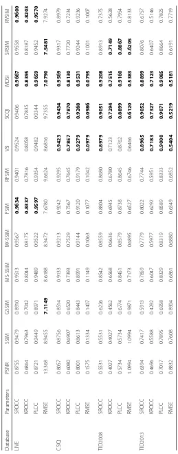
As described in Section2.2, the finalized splicing param-eters of the Log-Gabor filter bank are the number of scales nr = 5 and the number of orientationsnθ = 1.

Table 2 lists the SROCC/KROCC/PLCC/RMSE values obtained by applying the RVSIM index to the LIVE, CSIQ, TID2008, and TID2013 databases when different splicing parameters are taken to illustrate the rationality of the selection of these two parameters. The top performance is highlighted in bold. Table2shows that, when the number of scalesnr = 5 and the number of orientationsnθ = 1,

the RVSIM index exhibits its best performance.

4.2 Two sample examples

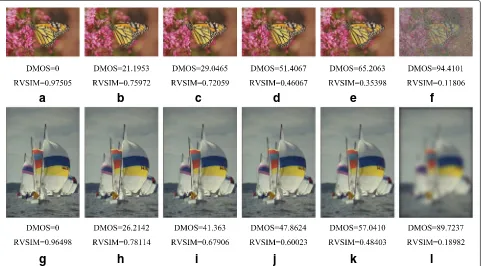
In order to determine whether the proposed RVSIM method agrees with human judgment, two sample images

(Fig. 7a,g, which are the same as Fig. 2f,l) in the LIVE database [45] are taken as examples. Corresponding to these two ground truth images, we select five noise-distorted images and five blur-noise-distorted images in differ-ent degrees from the LIVE database.

As shown in Fig. 7, images seem to degrade with increasing blur or noise from left to right. The LIVE database provides the difference mean opinion score (DMOS) for each image. A small DMOS represents a high-quality image. We calculate the objective scores of these images using the RVSIM method. The results can be found in Fig.7.

Figure 7 shows that RVSIM index is consistent with DMOS. This indicates that RVSIM method, in line with the subjective perception of HVS, can work well in indi-cating the image quality.

4.3 Performance comparison

(9)

(10)

a

b

c

d

e

f

g

h

i

j

k

l

Fig. 7Two group of images and their corresponding subjective/objective scores.a–fThe original imagemonarchand five noise-distorted images.

g–lThe original imagesailing2 and five blur-distorted images

the authors. Compared with traditional methods such as PSNR, SSIM, GSSIM, and MS-SSIM, RVSIM exhibits a good performance on the LIVE and CSIQ databases. As we only conduct the orthogonal experiments based on LIVE database, but do not carry out on TID2008 and TID2013 databases, RVSIM performs slightly worse than the best results on TID2008 and TID2013 databases.

Figure8 shows the scatter distributions of the subjec-tive DMOS versus the quality/distortion predicted scores by PSNR, SSIM, MS-SSIM, IW-SSIM, FSIM, SCQI, MDSI, RFSIM, and RVSIM indices on the LIVE database. Figure8

shows that the scatter plot of RVSIM is evenly distributed throughout the coordinate system and has a strong linear relationship with DMOS, which indicates that the RVSIM model has a strong congruency with HVS.

The experiments on these four databases (LIVE, CSIQ, TID2008, and TID2013) are insufficient to illustrate the problem. This study conducted gMAD competition in the Waterloo Exploration database to test the performance of RVSIM objectively and fairly.

Figure9shows the competition ranking in the Waterloo Exploration database. In the gMAD competition experi-ment, the results of the ranking of the 16 state-of-the-art methods have been provided by the official framework [60]. The experimenter is only allowed to participate in the competition ranking on the basis of 16 algorithms that have been provided. The algorithm to be added in

Fig.9a–fis RVSIM, SRSIM, RFSIM, VSI, MDSI, and SCQI respectively. Notably, the overall performance of RVSIM ranked first. In particular, the RVSIM performs consis-tently well in terms of aggressiveness, validating that it is a robust IQA method.

4.4 Discussion

In Table3, the top 6 methods are highlighted in bold, i.e., MDSI (16 times in bold), SCQI (12 times in bold), VSI (9 times in bold), SRSIM (4 times in bold), FSIM (3 times in bold), and RVSIM (3 times in bold). In Fig.9, the top 6 methods of the gMAD competition are RVSIM, SRSIM, MS-SSIM, MDSI, and RFSIM. The results are summarized in Table3and Fig.9, and the algorithm rank statistics are shown in Table4. The proposed RVSIM is highlighted in bold.

(11)

(12)

5 10 15 20 25 30 35 40 45 50

Objective score by PSNR

0 20 40 60 80 100 120

DMOS

Images in LIVE Curve fitted with logistic function

0 0.1 0.2 0.3 0.4 0.5 0.6 0.7 0.8 0.9 1

Objective score by SSIM

0 20 40 60 80 100 120

DMOS

0 0.1 0.2 0.3 0.4 0.5 0.6 0.7 0.8 0.9 1

Objective score by MS-SSIM

0 20 40 60 80 100 120

DMOS

0 0.1 0.2 0.3 0.4 0.5 0.6 0.7 0.8 0.9 1

Objective score by IW-SSIM

0 20 40 60 80 100 120

DMOS

0 0.1 0.2 0.3 0.4 0.5 0.6 0.7 0.8 0.9 1

Objective score by FSIM

0 20 40 60 80 100 120

DMOS

0.95 0.955 0.96 0.965 0.97 0.975 0.98 0.985 0.99 0.995 1

Objective score by SCQI

0 20 40 60 80 100 120

DMOS

0 0.1 0.2 0.3 0.4 0.5 0.6 0.7 0.8 0.9 1

Objective score by MDSI

0 20 40 60 80 100 120

DMOS

0 0.1 0.2 0.3 0.4 0.5 0.6 0.7 0.8 0.9 1

Objective score by RFSIM

0 20 40 60 80 100 120

DMOS

0 0.1 0.2 0.3 0.4 0.5 0.6 0.7 0.8 0.9 1

Objective score by RVSIM

0 20 40 60 80 100 120

DMOS

a

b

c

d

e

f

g

h

i

Fig. 8Scatter plots of predicted image quality indices on the LIVE database.aPSNR,bSSIM,cMS-SSIM,dIW-SSIM,eFSIM,fSCQI,gMDSI,hRFSIM,

andiRVSIM

MS-SSIM are not ranked at the top in indicator perfor-mance, they exhibited good results in gMAD competition. In particular, RVSIM had the highest rank in gMAD competition.

What results should be considered? The performance indices of the method and gMAD competition ranking are two kinds of judging basis. The performance indices can objectively reflect the performance of the method, but the benchmark databases only provide limited images because of the time-consuming and laborious subjec-tive scoring. gMAD competitions are performed between methods. The results of competitive ranking objectively reflect the relative performance of the IQA models. How-ever, the subjective scoring is needed because the Water-loo Exploration database is so large that the official did not

provide DMOS of the image in advance. In other words, they have both rationality and restrictions. A method which has both good results in performance indices and gMAD competitive ranking is considered as an excel-lent and more objective method. From this point of view, RVSIM exhibits a more consistent and stable performance than the other methods.

5 Conclusion

(13)

-0.6 -0.4 -0.2 0 0.2 0.4 0.6 0.8

Global ranking score

M3

DIIVINE NFERM BRISQUE BLIINDS-II

BIQI QAC TCLT LPSI SSIM PSNR NIQE ILNIQE FSIM

CORNIA MS-SSIM RVSIM

Resistance Aggressiveness

-0.6 -0.4 -0.2 0 0.2 0.4 0.6 0.8

M3

DIIVINE NFERMBLIINDS-II BRISQUE

CORNIA MS-SSIM SRSIM

-0.6 -0.4 -0.2 0 0.2 0.4 0.6

M3

DIIVINE NFERM

BLIINDS-II BRISQUE

CORNIA RFSIM MS-SSIM

-0.6 -0.4 -0.2 0 0.2 0.4 0.6

M3

DIIVINE NFERM

BLIINDS-II BRISQUE

CORNIA VSI

MS-SSIM

-0.6 -0.4 -0.2 0 0.2 0.4 0.6

M3

DIIVINE NFERM BRISQUE BLIINDS-II

CORNIA MDSI MS-SSIM

-0.6 -0.4 -0.2 0 0.2 0.4 0.6

M3

DIIVINE NFERMBLIINDS-II BRISQUE

BIQI SCQI QAC TCLT LPSI NIQE SSIM PSNR ILNIQE FSIM

CORNIA MS-SSIM

a

b

c

d

e

f

Fig. 9gMAD competition.aRVSIM,bSRSIM,cRFSIM,dVSI,eMDSI, andfSCQI

similarity matrix. Then, the MPC matrix is used to con-struct the pooling function and obtain the RVSIM index.

This study conducts experiments involving the RVSIM index on five benchmark IQA databases. The conclusion of the indicator performance indicates that the RVSIM index delivers a highly competitive prediction accuracy on the LIVE and CSIQ databases. The scatter plot of the sub-jective DMOS versus scores obtained by RVSIM predic-tion on the LIVE database suggests that the RVSIM model has a strong congruency with HVS. The conclusion of gMAD competition ranking on the Waterloo Exploration database implies that the performance of the RVSIM method is better than that of advanced IQA methods. The

Table 4Summary of the method rank statistics on five databases

LIVE, CSIQ, TID2008, TID2013, and Waterloo Exploration

Rank of indicators Methods Rank of competition Methods

1 MDSI 1 RVSIM

2 SCQI 2 SRSIM

3 VSI 3 MS-SSIM

4 SRSIM 4 VSI

5 FSIM 5 MDSI

6 RVSIM 6 RFSIM

The proposed RVSIM is highlighted in bold

overall performance on all five databases demonstrates that RVSIM is a robust IQA method.

Acknowledgements

The authors would like to thank Jiahua Cao and Associate Professor Weizheng Jin for the valuable opinions they had offered during our heated discussions.

Funding

This study is partially supported by National Natural Science Foundation of China (NSFC) (No. 61571334) and National High Technology Research and

Development Program (863 Program) (No. 2014AA09A512).

Availability of data and materials

The MATLAB source code of RVSIM can be downloaded athttps://sites.google.

com/site/jacobygy/for public use and evaluation. You can change this program as you like and use it anywhere, but please refer to its original source.

Authors’ contributions

GY conducted the experiments and drafted the manuscript. FL and YL implemented the core algorithm and performed the statistical analysis. DL designed the methodology. WY modified the manuscript. All authors read and approved the final manuscript.

Competing interests

The authors declare that they have no competing interests.

Publisher’s Note

Springer Nature remains neutral with regard to jurisdictional claims in published maps and institutional affiliations.

(14)

References

1. C Yan, H Xie, D Yang, J Yin, Y Zhang, Q Dai, Supervised hash coding with

deep neural network for environment perception of intelligent vehicles.

IEEE Trans. Intell. Transp. Syst.PP(99), 1–12 (2017).https://doi.org/10.

1109/TITS.2017.2749965

2. C Yan, Y Zhang, J Xu, F Dai, L Li, Q Dai, F Wu, A highly parallel framework

for HEVC coding unit partitioning tree decision on many-core processors.

IEEE Sig. Process Lett.21(5), 573–576 (2014)

3. C Yan, Y Zhang, J Xu, F Dai, J Zhang, Q Dai, F Wu, Efficient parallel

framework for HEVC motion estimation on many-core processors. IEEE

Trans. Circ. Syst. Video Technol.24(12), 2077–89 (2014)

4. Z Wang, EP Simoncelli, inHuman Vision and Electronic Imaging.

Reduced-reference image quality assessment using a wavelet-domain natural image statistic model, vol. 5666 (Proceedings of SPIE, San Jose, 2005), pp. 149–59

5. C Yan, H Xie, S Liu, J Yin, Y Zhang, Q Dai, Effective uyghur language text

detection in complex background images for traffic prompt

identification. IEEE Trans. Intell. Transp. Syst.PP(99), 1–10 (2017).

https://doi.org/10.1109/TITS.2017.2749977

6. G Xia, J Delon, Y Gousseau, Accurate junction detection and

characterization in natural images. Int. J. Comput. Vis.106(1), 31–56 (2014)

7. K Gu, G Zhai, X Yang, W Zhang, M Liu, in2013 IEEE International Conference

on Image Processing. Subjective and objective quality assessment for

images with contrast change (IEEE, Melbourne, 2013), pp. 383–87

8. J Ma, J Zhao, J Tian, AL Yuille, Z Tu, Robust point matching via vector field

consensus. IEEE Trans. Image Process.23(4), 1706–21 (2014)

9. W Zhang, A Borji, Z Wang, P Le Callet, H Liu, The application of visual

saliency models in objective image quality assessment: a statistical

evaluation. IEEE Trans. Neural Netw. Learn. Syst.27(6), 1266–78 (2016)

10. W Lin, C-CJ Kuo, Perceptual visual quality metrics: a survey. J. Vis.

Commun. Image Represent.22(4), 297–312 (2011)

11. Z Wang, AC Bovik, L Lu, inAcoustics, Speech, and Signal Processing (ICASSP),

2002 IEEE International Conference On, vol. 4. Why is image quality

assessment so difficult? (IEEE, Orlando, 2002), p. 3313

12. Z Wang, AC Bovik, HR Sheikh, EP Simoncelli, Image quality assessment: from error visibility to structural similarity. IEEE Trans. Image Process.

13(4), 600–12 (2004)

13. S-H Bae, M Kim, A novel image quality assessment with globally and locally consilient visual quality perception. IEEE Trans. Image Process.

25(5), 2392–2406 (2016)

14. K Gu, S Wang, H Yang, W Lin, G Zhai, X Yang, W Zhang, Saliency-guided

quality assessment of screen content images. IEEE Trans. Multimed.18(6),

1098–110 (2016)

15. A Rehman, Z Wang, Reduced-reference image quality assessment by

structural similarity estimation. IEEE Trans. Image Process.21(8), 3378–89

(2012)

16. J Farah, M-R Hojeij, J Chrabieh, F Dufaux, in2014 IEEE International

Conference on Acoustics, Speech and Signal Processing (ICASSP).

Full-reference and reduced-reference quality metrics based on sift (IEEE, Florence, 2014), pp. 161–165

17. S Xu, S Jiang, W Min, No-reference/blind image quality assessment: a

survey. IETE Tech. Rev.34(3), 223–45 (2017)

18. Z Wang, AC Bovik, Mean squared error: love it or leave it? a new look at

signal fidelity measures. IEEE Signal Proc. Mag.26(1), 98–117 (2009)

19. Z Wang, Applications of objective image quality assessment methods

[applications corner]. IEEE Signal Proc. Mag.28(6), 137–42 (2011)

20. Z Wang, AC Bovik, A universal image quality index. IEEE Sig. Process Lett.

9(3), 81–84 (2002)

21. Z Wang, EP Simoncelli, AC Bovik, inSignals, Systems and Computers, 2004.

Conference Record of the Thirty-Seventh Asilomar Conference On. Multiscale

structural similarity for image quality assessment, vol. 2 (IEEE, Florence, 2003), pp. 1398–402

22. G-H Chen, C-L Yang, L-M Po, S-L Xie, inAcoustics, Speech and Signal

Processing, 2006. ICASSP 2006 Proceedings. 2006 IEEE International

Conference On, vol. 2. Edge-based structural similarity for image quality

assessment (IEEE, Florence, 2006)

23. G-H Chen, C-L Yang, S-L Xie, inImage Processing, 2006 IEEE International

Conference On. Gradient-based structural similarity for image quality

assessment (IEEE, Atlanta, 2006), pp. 2929–32

24. C Li, AC Bovik, inIS&T/SPIE Electronic Imaging. Three-component weighted

structural similarity index (International Society for Optics and Photonics, San Jose, 2009), p. 72420

25. MP Sampat, Z Wang, S Gupta, AC Bovik, MK Markey, Complex wavelet structural similarity: a new image similarity index. IEEE Trans. Image

Process.18(11), 2385–401 (2009)

26. Z Wang, Q Li, Information content weighting for perceptual image quality

assessment. IEEE Trans. Image Process.20(5), 1185–98 (2011)

27. HR Sheikh, AC Bovik, G De Veciana, An information fidelity criterion for image quality assessment using natural scene statistics. IEEE Trans. Image

Process.14(12), 2117–28 (2005)

28. HR Sheikh, AC Bovik, Image information and visual quality. IEEE Trans.

Image Process.15(2), 430–44 (2006)

29. L Zhang, L Zhang, X Mou, D Zhang, FSIM: a feature similarity index for

image quality assessment. IEEE Trans. Image Process.20(8), 2378–86

(2011)

30. L Zhang, L Zhang, X Mou, inImage Processing (ICIP), 2010 17th IEEE

International Conference On. RFSIM: a feature based image quality

assessment metric using Riesz transforms (IEEE, Hong Kong, 2010), pp. 321–324

31. X-G Luo, H-J Wang, S Wang, Monogenic signal theory based feature similarity index for image quality assessment. AEU-International J.

Electron. Commun.69(1), 75–81 (2015)

32. P Cerejeiras, U Kähler,Monogenic signal theory. Oper. Theory. (Springer,

Basel, 2015), pp. 1701–1724

33. DJ Field, Relations between the statistics of natural images and the

response properties of cortical cells. JOSA A.4(12), 2379–94 (1987)

34. J Mannos, D Sakrison, The effects of a visual fidelity criterion of the

encoding of images. IEEE Trans. Inf. Theory.20(4), 525–36 (1974)

35. M Felsberg, G Sommer, The monogenic scale-space: a unifying approach to phase-based image processing in scale-space. J. Math. Imaging Vis.

21(1), 5–26 (2004)

36. C Zhao, J Wan, L Ren, Image feature extraction based on the two-dimensional empirical mode decomposition. Image Sig. Process

Congr.1, 627–31 (2008)

37. M Felsberg, G Sommer, The monogenic signal. IEEE Trans. Sig. Process.

49(12), 3136–44 (2001)

38. K Langley, SJ Anderson, The Riesz transform and simultaneous representations of phase, energy and orientation in spatial vision. Vis. Res.

50(17), 1748–65 (2010)

39. C Wachinger, T Klein, N Navab, The 2d analytic signal for envelope detection and feature extraction on ultrasound images. Med. Image Anal.

16(6), 1073–84 (2012)

40. L Wietzke, G Sommer, O Fleischmann, inComputer Vision and Pattern

Recognition, 2009. CVPR 2009. IEEE Conference On. The geometry of 2d

image signals (IEEE, Miami, 2009), pp. 1690–7

41. D Boukerroui, JA Noble, M Brady, On the choice of band-pass quadrature

filters. J. Math. Imaging Vis.21(1-2), 53–80 (2004)

42. JR Movellan, Tutorial on Gabor filters. Open Source Document (2002). http://mplab.ucsd.edu/tutorials/gabor.pdf. Accessed 24 July 2017 43. S Fischer, R Redondo, G Cristóbal, How to construct Log-Gabor filters.

Open Access Digit. CSIC Document.21, 1–9 (2009)

44. P Kovesi, What are Log-Gabor filters and why are they good? (2006). www.peterkovesi.com/matlabfns/PhaseCongruency/Docs/convexpl.

html. Accessed 24 July 2017

45. HR Sheikh, Z Wang, L Cormack, AC Bovik, LIVE image quality assessment

database release 2 (2005). [Online]. Available:http://live.ece.utexas.edu/

research/quality

46. P Kovesi, Phase congruency: a low-level image invariant. Psychol. Res.

64(2), 136–48 (2000)

47. P Kovesi, Image features from phase congruency. Videre: J. Comput. Vis.

Res.1(3), 1–26 (1999)

48. P Kovesi, inThe Australian Pattern Recognition Society Conference: DICTA

2003. Phase congruency detects corners and edges (The University of

Queensland, Sydney, 2003)

49. MN Gibbs, DJ MacKay, Variational Gaussian process classifiers. IEEE Trans.

Neural Netw.11(6), 1458–64 (2000)

50. Z Wang, AC Bovik, Modern image quality assessment. Synth. Lect. Image,

Video Multimed. Process.2(1), 1–156 (2006)

51. X Gao, W Lu, D Tao, X Li, inVisual Communications and Image Processing

2010. Image quality assessment and human visual system (International

Society for Optics and Photonics, Huangshan, 2010), p. 77440 52. DM Chandler, Seven challenges in image quality assessment: past,

(15)

53. K Gu, G Zhai, X Yang, W Zhang, in2014 IEEE International Conference on

Image Processing (ICIP). An efficient color image quality metric with

local-tuned-global model (IEEE, Paris, 2014), pp. 506–510

54. EC Larson, DM Chandler, Most apparent distortion: full-reference image

quality assessment and the role of strategy. J. Electron. Imaging.19(1),

011006 (2010)

55. N Ponomarenko, V Lukin, A Zelensky, K Egiazarian, M Carli, F Battisti, Tid2008-a database for evaluation of full-reference visual quality

assessment metrics. Adv. Mod. Radioelectron.10(4), 30–45 (2009)

56. N Ponomarenko, L Jin, O Ieremeiev, V Lukin, K Egiazarian, J Astola, B Vozel, K Chehdi, M Carli, F Battisti, et al., Image database tid2013: Peculiarities,

results and perspectives. Signal Process. Image Commun.30, 57–77 (2015)

57. K Ma, Z Duanmu, Q Wu, Z Wang, H Yong, H Li, L Zhang, Waterloo exploration database: New challenges for image quality assessment

models. IEEE Trans. Image Process.26(2), 1004–1016 (2017)

58. HR Sheikh, MF Sabir, AC Bovik, A statistical evaluation of recent full reference image quality assessment algorithms. IEEE Trans. Image

Process.15(11), 3440–51 (2006)

59. P Corriveau, A Webster, Final report from the video quality experts group on the validation of objective models of video quality assessment, phase II, Video Quality Experts Group, CO, USA, Tech. Rep. Phase II, (2003) 60. M Kede, W Qingbo, W Zhou, Z Duanmu, H Yong, H Li, Z Lei, Group MAD

competition—a new methodology to compare objective image quality models

61. L Zhang, Y Shen, H Li, VSI: a visual saliency-induced index for perceptual

image quality assessment. IEEE Trans. Image Process.23(10), 4270–81

(2014)

62. HZ Nafchi, A Shahkolaei, R Hedjam, M Cheriet, Mean deviation similarity index: efficient and reliable full-reference image quality evaluator. IEEE

Access.4, 5579–90 (2016)

63. L Zhang, H Li, inImage Processing (ICIP), 2012 19th IEEE International

Conference On. Sr-sim: A fast and high performance IQA index based on