O R I G I N A L A R T I C L E
Open Access
Parametric optimization of corrosion and wear of
electroless Ni-P-Cu coating using grey relational
coefficient coupled with weighted principal
component analysis
Supriyo Roy and Prasanta Sahoo
*Abstract
Background:This research article considers optimization of the four process parameters based on corrosion and wear of electroless Ni-P-Cu coatings. The major characteristics indexes for performance selected to evaluate the processes are corrosion potential (Ecorr), corrosion current density (Icorr) and wear. Among the corresponding four process parameters the first three are coating parameters,viz. concentration of nickel sulphate, concentration of sodium hypophosphite, concentration of copper sulphate and the fourth one is post deposition heat treatment temperature.
Methods:The corrosion property, i.e.EcorrandIcorr, has been studied by potentiodynamic polarization test and the wear is measured in terms of wear depth by DUCOM TR-25 multi-tribotester with block on roller arrangement. Results:In this study, the process is intrinsically combined with multiple performance indexes so that grey relational analysis is specially adopted to determine the optimal combination of coating parameters. Moreover, the weighted principal component analysis (WPCA) is applied to evaluate the weighting values corresponding to various performance characteristics so that their relative importance can be properly and objectively described. Conclusion:From the analysis the optimum combination of parameters for corrosion property and the optimum combination of parameters for corrosion and wear together are obtained. The chemical composition, surface morphology and phase behaviour are investigated using energy dispersive X-ray analysis, scanning electron microscopy and X-ray diffraction analysis, respectively.
Keywords:Ni-P-Cu; Corrosion; Wear; Grey relational coefficient; WPCA
Background
Coating is a method by which an artificial surface can be generated to the outer surface of the substrate material to protect it from corrosion and wear. These are the two deteriorating phenomena which are the source of major loss for industrial machinery. These not only reduce the life of the industrial components but also increase the maintenance cost and expenditure for replacement of parts. Since corrosion and wear both occur at the sur-face of the substrate, they can be reduced or eliminated by surface treatment. In this respect, the metallic surface
coating gives a practical solution. Electroless coating, also known as chemical or auto-catalytic coating, is a non-galvanic plating method that involves several simul-taneous chemical reactions in an aqueous solution, which occur without the use of external electrical power. That makes the difference of this process with that of conventional electroplating process which requires ex-ternal current source. Electroless coating process has gained wide acceptance in the market due to the excel-lent corrosion and wear resistance properties, and it is also good for soldering and brazing purposes (Sahoo and Das 2011). In recent days the binary electroless Ni-P coatings have become the research focus due to their * Correspondence:[email protected]
Department of Mechanical Engineering, Jadavpur University, Kolkata 700032, India
more superior properties. These properties can be fur-ther improved by incorporating a third particle into that binary alloy. The choice of the third particle depends on the desired property. Ternary Ni-P coatings, such as Ni-Cu-P (Yu et al. 2002; Aal and Aly 2009), Ni-W-P (Palaniappa and Seshadri 2008; Balaraju et al. 2006a; Balaraju et al. 2006b; Roy and Sahoo 2013; Roy and
Sahoo 2012), Ni-P-TiO2(Abdel Aal et al. 2008; Chen et
al. 2010; Novakovic and Vassiliou 2009), Ni-P-Al2O3
(Alirezaei et al. 2007; Balaraju et al. 2006c), Ni-P-PTFE (Ramalho and Miranda 2005; Huang et al. 2003) and Ni-P-SiC (Lin et al. 2006; Jiaqiang et al. 2006), have been prepared by electroless deposition. Among these ternary Ni-P alloy coatings, the electroless Ni-Cu-P alloy presents more superior corrosion resistance and thermal conductivity than the others (Liu et al. 2010; Valova et al. 2010; Liu and Zhao 2004; Wang et al. 1992). The inclusion of Cu in electroless Ni-P alloys improves their smoothness (Balaraju and Rajam 2005), brightness (Tarozaitë and Selskis 2006; Chen et al. 2006) and corrosion resistance (Liu and Zhao 2004; Zhao et al. 2004; Armyanov and Georgieva 2007). The crystallization behaviours of Ni-P-Cu coatings on aluminium substrates were investigated by Chen and Lin (1999). A comparative study on the crystallization
Table 1 Main coating parameters with their levels
Design factors Levels
1 2 3
Concentration of source of nickel (nickel sulphate solution) (g/l)
25 30 35
Concentration of reducing agent (sodium hypophosphite solution) (g/l)
10 15 20
Concentration of source of copper (copper sulphate) (g/l)
0.3 0.5 0.7
Heat treatment temperature (°C) 300 400 500
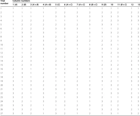
Table 2 L27orthogonal array
Trial number
Column numbers
1 (A) 2 (B) 3 (A×B) 4 (A×B) 5 (C) 6 (A×C) 7 (A×C) 8 (B×C) 9 (D) 10 11 (B×C) 12 13
1 1 1 1 1 1 1 1 1 1 1 1 1 1
2 1 1 1 1 2 2 2 2 2 2 2 2 2
3 1 1 1 1 3 3 3 3 3 3 3 3 3
4 1 2 2 2 1 1 1 2 2 2 3 3 3
5 1 2 2 2 2 2 2 3 3 3 1 1 1
6 1 2 2 2 3 3 3 1 1 1 2 2 2
7 1 3 3 3 1 1 1 3 3 3 2 2 2
8 1 3 3 3 2 2 2 1 1 1 3 3 3
9 1 3 3 3 3 3 3 2 2 2 1 1 1
10 2 1 2 3 1 2 3 1 2 3 1 2 3
11 2 1 2 3 2 3 1 2 3 1 2 3 1
12 2 1 2 3 3 1 2 3 1 2 3 1 2
13 2 2 3 1 1 2 3 2 3 1 3 1 2
14 2 2 3 1 2 3 1 3 1 2 1 2 3
15 2 2 3 1 3 1 2 1 2 3 2 3 1
16 2 3 1 2 1 2 3 3 1 2 2 3 1
17 2 3 1 2 2 3 1 1 2 3 3 1 2
18 2 3 1 2 3 1 2 2 3 1 1 2 3
19 3 1 3 2 1 3 2 1 3 2 1 3 2
20 3 1 3 2 2 1 3 2 1 3 2 1 3
21 3 1 3 2 3 2 1 3 2 1 3 2 1
22 3 2 1 3 1 3 2 2 1 3 3 2 1
23 3 2 1 3 2 1 3 3 2 1 1 3 2
24 3 2 1 3 3 2 1 1 3 2 2 1 3
25 3 3 2 1 1 3 2 3 2 1 2 1 3
26 3 3 2 1 2 1 3 1 3 2 3 2 1
behaviour of electroless Ni-P and Ni-Cu-P deposits was performed by Hui-Sheng et al. (2001) and found that the crystalline temperature for the formation of Ni3P
phase is higher for Ni-Cu-P coating than Ni-P coating. It was mentioned that the addition of copper into elec-troless Ni-P matrix could improve the corrosion resist-ance of the coatings (Mallory and Hadju 1991). The corrosion study of electroless Ni-P-Cu reveals that 90% Ni-7% Cu-3% P in 50% NaOH solution was better than that of as-plated Ni-P (Wang et al. 1992). The anticorro-sion properties of the Ni-Cu-P coatings in 1 M HCl, 1 M H2SO4and 3% NaCl solutions were investigated by Cissé
et al. (2010) using Tafel polarization curves and electro-chemical impedance spectroscopy. The result showed a mar-ginal improvement in corrosion resistance in 3% NaCl solution compared to acidic medium. As the corrosion and wear property of this coating depends on the coating parameters, the parameters can be optimized for best rosive media, i.e. NaCl solution. Practically, both the cor-rosion and wear take place simultaneously; hence, the parameters can be optimized taking the effect of corrosion and wear together. The Taguchi method is a statistical ap-proach for the purpose of designing and improving prod-uct quality. Tosun (2006) used the grey relational analysis for the determination of optimal drilling parameters with the objective of minimization of surface roughness and burr height. Deng (1982) proposed the grey system theory which has been proven to be useful for dealing with the problems with poor, insufficient and uncertain informa-tion. The grey-based Taguchi method was employed to optimize the process parameters of the submerged arc welding (SAW) in hardfacing, considering multiple weld qualities (Tarng et al. 2002). Grey relational analysis was adopted to investigate the electro discharge machining (EDM) parameters on machining Al-10% SiCp composites by Narender Singh et al. (2004). Several researchers have used grey relational method to optimize the design process parameters, but most of the researchers have selected the weighting values of the response parameters according to their own estimation during calculation of the grey relational grade. This method cannot emphasize the relative importance of the response parameters related with the experiment. The case study by Antony (2000) demonstrates the potential of multi-response optimization in industrial experiments using Taguchi's quality loss func-tion and principal component analysis. The research of Lua et al. (2009) about the optimization problem with multiple performance characteristics using grey relational analysis presents a remedy by calculating the correspond-ing weightcorrespond-ing values uscorrespond-ing principal component analysis (Hotelling 1993). The researchers have used grey relational analysis for optimizing combination of cutting parameters and principal component analysis for determining the corresponding weighting values of various performance
characteristics. In this present investigation, the optimum combination of parameters for corrosion and wear, the grey relational coefficient is used and the corresponding weigh-ing value of each performance characteristics calculated by weighted principal component analysis considering the grey relational coefficients and the effect of all responses are clubbed together into multiple performance index. The sur-face morphology, chemical composition and phase trans-formation behaviour were studied by scanning electron microscopy (SEM), energy dispersive X-ray spectroscopy (EDX) and X-ray diffraction (XRD) analyses, respectively.
Methods
Selection of parameters
The electroless coatings involve large number of process parameters which can affect the performance character-istics of the coatings. In this present study, after a large number of literature review and experimental trials, four main process parameters have been selected as input pa-rameters. Among the four parameters the first three are coating parameters, viz. concentration of nickel sulphate (source of nickel), concentration of sodium hypophosphite (reducing agent) and concentration of copper sulphate (source of copper), and the fourth one is the post-deposition heat treatment temperature. The operating
Table 3 Electroless bath constituents
Parameters Values
Nickel sulphate (g/l) 25 to 35
Sodium hypophosphite (g/l) 10 to 20
Sodium citrate (g/l) 15
Copper sulphate (g/l) 0.3 to 0.7
pH 9.5
Temperature (°C) 85
Duration of coating (h) 2
Bath volume (ml) 200
range of the parameters has been selected on the ex-perimental basis, within which the coating can be de-posited. The range of each parameter has been divided in to three equally spaced levels. The main parameters with their values are shown in Table 1. The responses are corrosion potential, corrosion current density and wear depth.
Experimental design
This experimental investigation consists of four three-level input parameters; hence, with all possible combi-nations, a total number of (3)4= 81 experiments can be carried out. To save time and cost, the number of experi-ments has been reduced by using Taguchi's specially developed orthogonal array (OA). The selection of OA depends on the number of individual parameters and their interaction considered for the analysis. In this study along with four individual parameters, the interac-tions between three coating parameters, i.e. interaction between nickel sulphate and sodium hypophosphite, sodium hypophosphite and copper sulphate, and nickel sulphate and copper sulphate, have been considered. As this is a three-level experiment, the total degrees of free-dom associated with this experiment is 20. Hence a stand-ard L27 OA has been selected as this has 26 degrees
of freedom which is higher than the degrees of freedom of experiment. A standard L27OA is shown in Table 2,
which consists of 27 rows and 13 columns. Each row represents the combination of parameters for deposition of coating, and each column indicates the individual factors and their interactions.
Results and discussion Coating deposition
Mild steel blocks (AISI 1040) of size 20 mm × 20 mm × 8 mm are used as substrates for the deposition of elec-troless Ni-P-Cu coating. This particular dimension of the sample is chosen to fit the counter part of block on roller multi-tribotester apparatus. The sample is mech-anically cleaned from foreign matters and corrosion products. After that, the MS sample is cleaned using dis-tilled water. Then, a pickling treatment is given to the specimen with dilute (50%) hydrochloric acid for 1 min to remove any surface layer formed like rust followed by rinsing in distilled water and methanol cleaning. Table 3 indicates the bath composition and the operating conditions for successful coating of electroless Ni-P-Cu.
Figure 2Block on roller arrangement for wear test.
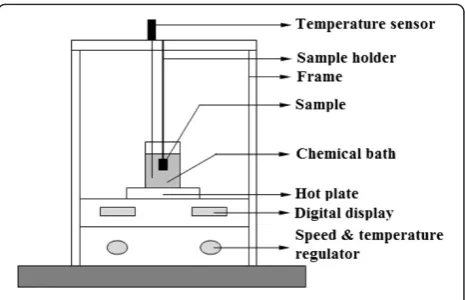
Nickel sulphate is used as the source of nickel while so-dium hypophosphite is the reducing agent and soso-dium citrate was added as complexing agent. The bath is pre-pared by adding the constituents in appropriate se-quence. The pH of the solution is maintained around 9.5 by continuous monitoring with a pH meter. The cleaned samples are activated in palladium chloride solution at a temperature of 55°C. Activated samples are then sub-merged into the electroless bath which is maintained at a temperature of 85°C with the help of a hot plate cum stirrer attached with a temperature sensor also sub-merged in the solution. The deposition is carried out for 2 h. The range of coating thickness is found to lie around 28 to 30μm by measuring with a digital micrometer in-strument. After deposition, the samples are taken out of the bath and heat-treated according to the experimental design. Figure 1 shows the schematic diagram of coating deposition set-up.
Wear measurement
The wear depths of heat-treated Ni-P-Cu-coated speci-mens are measured under non-lubricated condition using a multi-tribotester with block on roller configur-ation (DUCOM TR-25, Bangalore, Karnataka, India). The Ni-P-Cu-coated specimens serve as test specimens of average hardness of 42 HRc, which are held horizon-tally against a rotating roller coated with titanium nitride of hardness 85 HRc of 50-mm diameter × 20-mm thick-ness, as shown in Figure 2. As the hardness of the roller is higher than the hardness of coating, it may be assured that the wear will take place on the coating only. The wear test of each specimen is carried out for 5 min with 25 N load at a speed of 50 rpm. Dead weights are placed on the loading platform which is attached at one end of a 1:5 ratio loading lever. A linear voltage resistance transducer is used for measuring wear in terms of wear depth. It is worth noting that, in general, wear is mea-sured in terms of wear volume or mass loss. However, in the present case, wear is expressed in terms of displace-ment or wear depth. Hence, to ensure that the wear measurements are accurate, the wear depth results are compared with the weight loss of the specimens and al-most linear relationship is observed between the two for the range of test parameters considered in the present study.
Polarization study
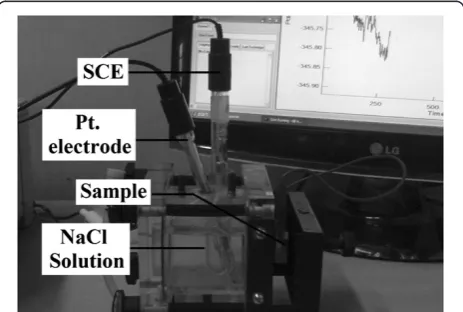
The potentiodynamic polarization tests of heat-treated Ni-P-Cu coatings are carried out using a potentiostat (Gill AC) of ACM Instruments, UK, shown in Figure 3. The corrosion parameters were measured by potentiody-namic polarization curve measurements. The tests are
conducted at an ambient temperature of about 25°C with 3.5% sodium chloride solution as the electrolyte. The electrochemical cell consists of three electrodes. The coated specimen forms the working electrode which is actually the sample being interrogated. A saturated calomel electrode (SCE) forms the reference electrode which provides a stable ‘reference’against which the ap-plied potential may be accurately measured. A platinum electrode serves as the counter electrode which provides the path for the applied current into the solution. The design of the cell kit is such that only an area of 1 cm2 of the coated surface is exposed to the electrolyte. The experimental set-up is shown in Figure 1. A settling time of 15 min is assigned before every experiment in order to stabilize the open circuit potential (OCP). The poten-tiostat is controlled via a PC which also captures the polarization data. Potentiodynamic polarization studies were carried out by polarizing the working electrode
Table 4 Results of corrosion and wear test
Experiment number Ecorr(mV vs. SCE) Icorr(μA/cm2) Wear (μm)
1 −353.66 0.191 18.98
2 −233.31 0.7903 26.6168
3 −369.54 4.651 11.5636
4 −231.58 0.1379 10.4644
5 −304.83 0.6771 4.3218
6 −526.89 8.627 13.0348
7 −434.42 1.104 20.4475
8 −256.26 0.7201 15.979
9 −417.6 1.264 9.3686
10 −583.88 1.7968 9.7621
11 −434.89 0.9978 13.653
12 −558.04 4.3578 18.1084
13 −346.32 2.533 14.6986
14 −443.27 0.8437 1.432
15 −458.24 5.135 18.086
16 −434.01 0.2643 25.949
17 −528.22 2.6583 25.3954
18 −461.35 5.009 14.3488
19 −576.21 5.0188 11.369
20 −601.63 3.822 1.4966
21 −437.01 8.118 25.32
22 −559.43 3.84 18.414
23 −484.94 9.864 17.4277
24 −563.11 0.77731 13.9094
25 −523.09 5.231 16.5901
26 −466.68 7.961 13.4266
from the OCP to 250 mV in cathodic direction and 250 mV in anodic direction at a scan rate of 1 mV/s. The corrosion current densities (Icorr) were determined
by extrapolating the straight-line section of the anodic and cathodic branches of the Tafel plots in the vicinity of the corrosion potential using the software installed in the instrument The polarization plot is obtained from the dedicated software, which also possesses a special tool in order to manually extrapolate the values of Ecorr
(corrosion potential) andIcorr(corrosion current density)
from the plot. Each experiment has been repeated for
three times, and the variation of result was within 2%. The average value has been taken for analysis. The re-sults of wear and corrosion are shown in Table 4. The Tafel plots and the variation of wear are shown in Figure 4
Characterization of coating
The characterization of the coating is necessary so that it can be made sure that the coating is properly devel-oped. Energy dispersive X-ray analysis (EDAX Corpor-ation, Mahwah, NJ, USA) is performed to determine the
Figure 4Tafel plots and variation of wear depths.For different compositions of Ni at different heat treatment temperatures(a)300°C,(b)
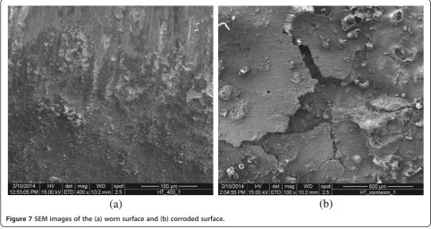
composition of the coating in terms of the weight per-centages of nickel, phosphorous and copper. Figure 5 shows the EDX spectra of the coated surface. From the analysis, it is found that the coating consists of 11% P, 4% Cu and the remaining is Ni. Figure 6 shows the SEM of as-deposited and heat-treated (300°C, 400°C, 500°C) Ni-P-Cu-coated surface. A deposit coarse nodular struc-ture without any porosity in as-deposited condition is clear. Nodular deposition in a coating depends on nu-cleation rate and the growth of the deposit. Nunu-cleation rate depends on the bath constituents and the operat-ing condition of the experiment. From the figures, it is clear that due to heating, crack appears in the coating. Figure 7 shows the image of the worn surface and the corroded surface. The phase transformation behaviour has been studied by XRD. Figure 8 shows the XRD pat-tern of as-deposited and heat-treated condition. From the figure, it is clear that in as-deposited condition the coating is mostly amorphous, but crystalline peaks ap-pear after heating. The major crystalline peaks of Ni, Cu3P, Ni3P and Ni3P2appear after heating at 400°C for
1 h.
Analysis methodology and discussion Grey relational coefficient
In this study among the three responses, a higher value of corrosion potential (Ecorr) and a lower value of
corro-sion current density (Icorr) are desired for good corrosion
resistance and obviously a lower value of wear depth has been targeted. As there is a huge difference between the average value of each response, the result obtained from
the analysis considering these values may not give the correct result when the effect of all the parameters are considered together. To eliminate this effect, the result data of each response have been normalized or scaled between 0 and 1. The value 1 represents a good result and 0 represents a worse result. Here,Ecorris normalized
considering the bigger the better as a higher corrosion potential indicates good corrosion resistance. The Icorr
and wear depth both are normalized considering the smaller the better. Using this normalized value, the grey relational coefficients are calculated, which are explained stepwise:
Step 1: normalization Normalization ofEcorris performed
using Equation 1:
Normalized value of Ecorr Ej ¼
Ej−Emin
Emax−Emin ð
1Þ
Normalization ofIcorrand wear depth is performed using
Equations 2 and 3:
Normalized value of Icorr Ij ¼
Imax−Ij
Imax−Imin ð
2Þ
Normalized value of W W j¼ Wmax−Wj Wmax−Wmin; ð
3Þ
whereEj=Ecorrvalue corresponding to thejth experiment
Ij=Icorrvalue corresponding to thejth experiment
Wj= wear value corresponding to thejth experiment j= sequence of experimental run (j= 1, 2, 3…); as there is a total of 27 experimental runs, the maximum value ofjis 27.
Step 2: grey relational generation The grey relational coefficient (gj) for each response has been generated using Equation 4:
gj¼ΔRminþrΔRmax
ΔR
j þrΔRmax
ð4Þ
whereR
j = the normalized response value (Ej for
cor-rosion potential, Ij for corrosion current and Wj for
wear depth)
ΔR
j ¼Rjmax−Rj;
R
jmax¼the maximum value ofRj
ΔR
max and ΔRmin are the maximum and minimum values ofΔRj, respectively.
Figure 7SEM images of the (a) worn surface and (b) corroded surface.
r is a distinguishing coefficient, which belongs to [0, 1]. The distinguishing coefficient weakens the effect of max ΔRmaxwhen it gets too big, enlarging the different
significance of the relational coefficient. The suggested value of the distinguishing coefficient, r, is 0.5, due to the moderate distinguishing effects and good stability of outcomes. Therefore,ris adopted as 0.5 for further ana-lysis in the present case.
The normalized values and grey relational coeffi-cients of each response are shown in Table 5. The
conventional method for finding the grey relational grade is to take the average of these grey relational co-efficients, i.e. considering equal contribution of each response to the overall variation. However, the eigen-value of a principal component gives a fairly good idea about the variance of the original variables that can be explained by the principal component. A larger ei-genvalue of a principal component implies that the
Table 5 Results of grey analysis
Experiment number
Normalized value Δvalue Grey coefficient
Ecorr Icorr Wear Ecorr Icorr Wear Ecorr Icorr Wear
1 0.67010 0.99454 0.30323 0.32990 0.00546 0.69677 0.60248 0.98920 0.41779
2 0.99532 0.93292 0.00000 0.00468 0.06708 1.00000 0.99074 0.88171 0.33333
3 0.62719 0.53598 0.59771 0.37281 0.46402 0.40229 0.57286 0.51866 0.55415
4 1.00000 1.00000 0.64136 0.00000 0.00000 0.35864 1.00000 1.00000 0.58231
5 0.80205 0.94456 0.88526 0.19795 0.05544 0.11474 0.71639 0.90019 0.81335
6 0.20197 0.12718 0.53929 0.79803 0.87282 0.46071 0.38520 0.36421 0.52045
7 0.45186 0.90067 0.24496 0.54814 0.09933 0.75504 0.47703 0.83426 0.39839
8 0.93331 0.94014 0.42239 0.06669 0.05986 0.57761 0.88231 0.89308 0.46399
9 0.49731 0.88422 0.68487 0.50269 0.11578 0.31513 0.49866 0.81198 0.61340
10 0.04797 0.82944 0.66924 0.95203 0.17056 0.33076 0.34434 0.74564 0.60186
11 0.45059 0.91159 0.51475 0.54941 0.08841 0.48525 0.47646 0.84975 0.50748
12 0.11779 0.56613 0.33784 0.88221 0.43387 0.66216 0.36174 0.53540 0.43023
13 0.68993 0.75375 0.47323 0.31007 0.24625 0.52677 0.61723 0.67001 0.48696
14 0.42794 0.92743 1.00000 0.57206 0.07257 0.00000 0.46639 0.87326 1.00000
15 0.38749 0.48622 0.33873 0.61251 0.51378 0.66127 0.44943 0.49320 0.43056
16 0.45297 0.98700 0.02652 0.54703 0.01300 0.97348 0.47754 0.97467 0.33933
17 0.19838 0.74086 0.04850 0.80162 0.25914 0.95150 0.38414 0.65864 0.34447
18 0.37908 0.49917 0.48712 0.62092 0.50083 0.51288 0.44606 0.49959 0.49364
19 0.06869 0.49816 0.60544 0.93131 0.50184 0.39456 0.34933 0.49908 0.55893
20 0.00000 0.62122 0.99743 1.00000 0.37878 0.00257 0.33333 0.56897 0.99490
21 0.44486 0.17952 0.05149 0.55514 0.82048 0.94851 0.47387 0.37865 0.34518
22 0.11404 0.61936 0.32570 0.88596 0.38064 0.67430 0.36076 0.56777 0.42579
23 0.31534 0.00000 0.36487 0.68466 1.00000 0.63513 0.42206 0.33333 0.44048
24 0.10409 0.93426 0.50457 0.89591 0.06574 0.49543 0.35819 0.88380 0.50229
25 0.21224 0.47635 0.39813 0.78776 0.52365 0.60187 0.38827 0.48845 0.45377
26 0.36468 0.19566 0.52374 0.63532 0.80434 0.47626 0.44040 0.38334 0.51216
27 0.29855 0.77647 0.64940 0.70145 0.22353 0.35060 0.41617 0.69105 0.58782
Table 6 Results obtained consideringEcorrandIcorr
Principal components
Eigenvalue Proportion of overall variation
Eigenvector
1st 1.5401 0.77 [0.707, 0.707]
2nd 0.4599 0.23 [0.707,−0.707]
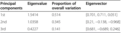
Table 7 Results obtained consideringEcorr,Icorrand wear
Principal components
Eigenvalue Proportion of overall variation
Eigenvector
1st 1.5414 0.514 [0.701, 0.711, 0.051]
2nd 1.0358 0.345 [0.21,−0.138,−0.968]
component's contribution in explaining the overall vari-ation is higher. In this study, the corresponding weight-ing values are obtained from the principal component analysis.
Weighted principal component analysis
According to Antony (2000), the components with ei-genvalues greater than 1 may be selected to replace the original responses. However, problems can arise in the situations where more than one eigenvalue becomes greater than 1. The weighted principal component (WPC)-based procedure (Su and Tong 1997; Liao 2006) for optimization of multi-response processes makes use of all the principal components irrespective of the eigen-values so that the overall variation in all the responses can be completely explained. In this approach, the proportion
of overall variation explained by each component is treated as the weight to combine all the principal com-ponents in order to form a multi-response perform-ance index (MPI). Then, the best combination of the parametric settings can easily be obtained which can optimize the MPI. The procedure for calculating MPI is described stepwise:
Table 8 Results obtained consideringEcorrandIcorr
Experiment number
Principal component MPI
P1 P2
1 1.12532 −0.27341 0.80361
2 1.32382 0.07708 1.03707
3 0.77171 0.03832 0.60303
4 1.41400 0.00000 1.08878
5 1.14292 −0.12995 0.85016
6 0.52984 0.01484 0.41139
7 0.92709 −0.25256 0.65577
8 1.25520 −0.00761 0.96475
9 0.92662 −0.22152 0.66255
10 0.77062 −0.28372 0.52812
11 0.93763 −0.26391 0.66127
12 0.63428 −0.12278 0.46016
13 0.91008 −0.03731 0.69218
14 0.94713 −0.28765 0.66313
15 0.66644 −0.03094 0.50604
16 1.02671 −0.35147 0.70973
17 0.73724 −0.19408 0.52304
18 0.66857 −0.03784 0.50610
19 0.59983 −0.10588 0.43752
20 0.63793 −0.16659 0.45289
21 0.60273 0.06732 0.47959
22 0.65647 −0.14636 0.47182
23 0.53406 0.06273 0.42566
24 0.87808 −0.37160 0.59066
25 0.61984 −0.07082 0.46099
26 0.58238 0.04035 0.45772
27 0.78280 −0.19435 0.55806
Table 9 Results obtained consideringEcorr,Icorrand wear
Experiment number
Principal components MPI
P1 P2 P3
1 1.14697 −0.41441 −0.16849 0.42281
2 1.33841 −0.23629 0.14919 0.62746
3 0.79860 −0.48769 0.16908 0.26607
4 1.44170 −0.49168 0.13525 0.59047
5 1.18370 −0.76110 0.06771 0.35539
6 0.55552 −0.47317 0.13941 0.14195
7 0.94788 −0.40060 −0.15194 0.32758
8 1.27714 −0.38710 0.09966 0.53695
9 0.95816 −0.60110 −0.06897 0.27539
10 0.80223 −0.61319 −0.13119 0.18230
11 0.96405 −0.50845 −0.13617 0.30090
12 0.65619 −0.41439 −0.01671 0.19196
13 0.93389 −0.43422 0.07849 0.34128
14 0.99883 −0.99057 −0.03806 0.16629
15 0.68768 −0.39047 0.07217 0.22893
16 1.04505 −0.36269 −0.26287 0.37496
17 0.75514 −0.34367 −0.10747 0.25442
18 0.69307 −0.45311 0.08099 0.21133
19 0.62824 −0.53656 0.03152 0.14224
20 0.68894 −0.97158 0.07973 0.03016
21 0.61901 −0.28688 0.14673 0.23989
22 0.67829 −0.41475 −0.04077 0.19980
23 0.55533 −0.38375 0.16611 0.17647
24 0.90509 −0.53296 −0.24144 0.24730
25 0.64261 −0.42512 0.03950 0.18920
26 0.60740 −0.45618 0.16179 0.17763
27 0.81305 −0.57698 −0.04812 0.21206
Table 10 Response table consideringEcorrandIcorr
Parameters Level Deviation
1 2 3
A 0.7863 0.5833 0.4817 0.3047
B 0.607 0.6333 0.611 0.0263
C 0.6498 0.6706 0.5308 0.1398
Step 1: eigenvalue and eigenvectors and proportion of overall variance The eigenvalue (λ) and eigenvectors (V) are calculated from Equation 5 imposing a condition
XQ
k¼1 V2
k ¼1
G−λI
½ ½ ¼V 0 ð5Þ
where
G¼
var 1ð Þ cov 1ð ;2Þ … cov 1ð ;kÞ cov 2ð ;1Þ var 2ð Þ … cov 2ð ;kÞ
… … … …
covð Þj;1 covðR;2Þ … varðR;kÞ 2
6 6 4
3 7 7 5
is the covariance matrix of grey relational coefficients.
kis the number of quality characteristics; in this prob-lem, the maximum value ofkis 3.
The proportion of overall variance or weight is calcu-lated using Equation 6:
Wk ¼ λk
XQ
k¼1
λk
ð6Þ
The eigenvalues, eigenvectors and proportion of over-all variance considering only corrosion parameters (Ecorr
and Icorr) are shown in Table 6, and the corresponding
values considering both corrosion and wear (Ecorr, Icorr
andW) are shown in Table 7.
Step 2: calculation of principal components and MPI The principal components are calculated using Equation 7:
P
½ ¼½ g ½ V ð7Þ
The MPI is calculated using Equation 8:
MPI¼X
Q
k¼1
Pj;kWk;1 ð8Þ
The principal components and MPI considering only corrosion parameters (Ecorr and Icorr) are shown in
Table 8, and the corresponding values considering both corrosion and wear (Ecorr, Icorr and W) are shown in
Table 9.
Optimum combination of parameters
As the design of experiment is orthogonal, the effect of each parameter on MPI can be separated out by taking the average of same levels of each input parameter. For example, among the 27 experiments, there are 9 experi-ments, which include the level 1 of parameter A. Taking the average of these 9 MPI values, the mean MPI of level 1 for parameter Acan be calculated. Similar procedure is applicable for other parameters. Table 10 shows the mean response table of the MPI taking only corrosion parame-ters (corrosion potential and corrosion current density), and Table 11 shows the same considering all the three parameters (corrosion potential, corrosion current and wear depth). Figures 9 and 10 show the main effect plots obtained from the response tables, respectively. From the plots, the optimum combination of input parameters can be obtained. As the larger value of MPI corresponds better multiple response characteristics, the optimum combination can be obtained by selecting the largest level average of each parameter. Figure 9 yields the optimum combination considering only corrosion parameters is A1B2C2D2, and Figure 10 yields the optimum combin-ation considering corrosion parameters and wear together is A1B3C1D2.
Table 11 Response table consideringEcorr,Icorrand wear
Parameters Level Deviation
1 2 3
A 0.3938 0.2503 0.1794 0.2144
B 0.2671 0.272 0.2844 0.0173
C 0.3079 0.2917 0.2239 0.084
D 0.253 0.3072 0.2633 0.0542
Significance of parameters on MPI
The response table also reveals the significance of each individual factor. In the response tables, the maximum deviation of each parameter is listed in the right column. It is obtained by subtracting the lowest mean MPI from the largest mean MPI value among the three levels of any parameter. The parameter has huge impact on the multiple responses, which has maximum deviation. From the tables, it is clear that parameterA, i.e. concen-tration of nickel sulphate, and parameter C, i.e. concen-tration of copper sulphate, have positive impact on the corrosion and wear property. The effect of nickel is highly dominant for both the cases, but the effect of copper is higher when only corrosion parameters are considered. It has been seen that due to heat treatment the structure of the coating transforms into crystalline. The coating becomes hard mainly due to the formation of the nickel phosphide structure at 400°C, and thus, im-proved wear resistance is achieved at this stage along with the corrosion. According to Hui-Sheng et al. (2001), after heating 500°C for 1 h, the metastable phase Ni5P2transforms completely to stable Ni3P phase. It leads
to harder and wear resistant coating due to crystallization which leads to more corrosive prone surface. Thus, 500°C may not be the optimum heat treatment temperature. Hence, this present analysis has a good agreement with this result. The results of analysis of variance (ANOVA) considering the corrosion parameters (EcorrandIcorr) and
also considering the corrosion parameters and wear
together are shown in Tables 12 and 13, respectively. The tables reveal that the percentage contribution of nickel is highest for both the conditions. Along with this the ANOVA results also focus on the significance of the inter-action of parameters on the responses. It is clear from both the ANOVA tables that the percentage contribution of the interaction between nickel and copper is highest among the three interactions.
Confirmation test
To validate the result obtained from the analysis, a con-firmation test was carried out with the optimum com-bination of parameters. Coatings are developed with the optimum combination of parameters obtained from optimization analysis, viz. A1B2C2D2 for corrosion optimization and A1B3C1D2 for combined corrosion and wear optimization. These coatings are then sub-jected to corrosion and wear tests. The results of these tests are compared with the tests on coatings devel-oped with mid-level combination of parameters, i.e. A2B2C2D2. It is because with this combination the bath is most stable for a long time, and maximum thickness of coating can be achieved. However, the aim is to find out the best quality coating against corrosion and wear. Hence, a comparison between the mid-level result and the optimum level results has been carried out. The result of the confirmation test is tabulated in Table 14. From the table, it is clear that at optimum condition for corrosion, the value of corrosion potential is
Figure 10Main effect plot consideringEcorr,Icorrand wear.
Table 12 ANOVA table consideringEcorrandIcorr
Source df SS MS F P
A 2 0.43318 0.21659 11.77 46.62
B 2 0.00362 0.00181 0.1 0.39
C 2 0.1024 0.0512 2.78 11.02
D 2 0.00425 0.00213 0.12 0.46
A×B 4 0.01109 0.00277 0.15 1.19
A×C 4 0.20227 0.05057 2.75 21.77
B×C 4 0.06183 0.01546 0.84 6.65
Error 6 0.11043 0.01841 11.89
Total 26 0.92908 100.00
Table 13 ANOVA table consideringEcorr,Icorrand wear
Source df SS MS F P
A 2 0.214715 0.107358 11.74 42.44
B 2 0.001432 0.000716 0.08 0.28
C 2 0.03575 0.017875 1.95 7.07
D 2 0.014896 0.007448 0.81 2.94
A×B 4 0.021066 0.005266 0.58 4.16
A×C 4 0.122368 0.030592 3.34 24.19
B×C 4 0.040801 0.0102 1.12 8.06
Error 6 0.054888 0.009148 10.85
improved by 49%, while the value of corrosion current de-creases by 84%. For combined corrosion and wear optimization case, the value of corrosion potential is im-proved by 7%, while the value of corrosion current de-creases by 76% and wear depth dede-creases by 40%. Thus, the optimum combination of parameters yields a better coating. The polarization curves for both the optimum conditions and mid-level combination are shown in Figure 11. The improvement of corrosion resistance of the coatings obtained from the optimum combination of pa-rameters is clearly seen in these plots since corrosion po-tential increases and corrosion current decreases from the mid-level combination.
Conclusions
The electroless ternary Ni-P-Cu coating has been devel-oped on mild steel substrate by varying four input design parameters, namely concentration of nickel source (nickel sulphate), concentration of reducing agent (sodium hypo-phosphite), concentration of copper source (copper sulphate) and post-deposition heat treatment temperature. The design of experiment was done by Taguchi L27OA with
27 experimental runs. The wear depth of the heat-treated coatings was measured with a multi-tribotester instrument with block on roller configuration. The polarization (corrosion) tests were carried out using a potentiostat instrument. By extrapolating the Tafel plot, the corro-sion current density and the corrocorro-sion potential were measured. Then, the grey analysis together with weighted principal component analysis is successfully employed for finding out the optimal combinations of the design process parameters of electroless Ni-P-Cu coatings for better value of polarization test and also considering the polarization and wear test together. Confirmation tests were carried out for both the cases to validate the experimental value. The energy dispersive X-ray analysis shows that it is a pure tern-ary coating consisting of nickel phosphorous and copper; the surface morphology and phase transformation behaviour have been studied by SEM and XRD analyses, respectively.
Competing interests
The authors declare that they have no competing interests.
Authors’contributions
SR carried out the experiments, analysed the data and drafted the manuscript. PS supervised the experiments, monitored the analysis and corrected the manuscript. Both authors read and approved the final manuscript.
Received: 23 May 2014 Accepted: 14 July 2014
References
Sahoo, P, & Das, SK. (2011). Tribology of electroless nickel coatings–a review.
Materials and Design, 32, 1760–1775.
Yu, H, Sun, X, Luo, SF, Wang, YR, & Wu, ZQ. (2002). Multifractal spectra of atomic force microscope images of amorphous electroless Ni-P-Cu alloy.Applied Surface Science, 191, 123–127.
Aal, AA, & Aly, MS. (2009). Electroless Ni–Cu–P plating onto open cell stainless steel foam.Applied Surface Science, 255, 6652–6655.
Palaniappa, M, & Seshadri, SK. (2008). Friction and wear behaviour of electroless Ni-P and Ni-W-P alloy coatings.Wear, 26, 735–740.
Balaraju, JN, Jahan, SM, & Rajam, KS. (2006a). Studies on autocatalytic deposition of ternary Ni–W–P alloys using nickel sulphamate bath.Surface and Coatings Technology, 201, 507–512.
Balaraju, JN, Anandan, C, & Rajam, KS. (2006b). Influence of codeposition of copper on the structure and morphology of electroless Ni–W–P alloys from sulphate- and chloride-based baths.Surface and Coatings Technology, 200, 3675–3681. Roy, S, & Sahoo, P. (2013). Tribological performance optimization of electroless
Ni-P-W coating using weighted principal component analysis.Tribology in Industry, 35(4), 297–307.
Roy, S, & Sahoo, P. (2012). Corrosion study of electroless Ni-P-W coatings using electrochemical impedance spectroscopy.Portugaliae Electrochimica Acta, 30(3), 203–220.
Abdel Aal, A, B. Hassan, H, & Abdel Rahim, MA. (2008). Nanostructured Ni–P–TiO2 composite coatings for electrocatalytic oxidation of small organic molecules.
Journal of Electroanalytical Chemistry, 619–620, 17–25.
Chen, W, Gao, W, & He, Y. (2010). A novel electroless plating of Ni–P–TiO2 nano-composite coatings.Surface & Coatings Technology, 204, 2493–2498. Novakovic, J, & Vassiliou, P. (2009). Vacuum thermal treated electroless NiP–TiO2
composite coatings.Electrochimica Acta, 54, 2499–2503.
Alirezaei, S, Monirvaghefi, SM, Salehi, M, & Saatchi, A. (2007). Wear behavior of Ni–P and Ni–P–Al2O3electroless coatings.Wear, 262, 978–985. Balaraju, JN, Kalavati, & Rajam, KS. (2006c). Influence of particle size on the
microstructure, hardness and corrosion resistance of electroless Ni–P–Al2O3 composite coatings.Surface & Coatings Technology, 200, 3933–3941. Ramalho, A, & Miranda, JC. (2005). Friction and wear of electroless NiP and NiP + PTFE
coatings.Wear, 259, 828–834. Figure 11Tafel plots.Mid-level combination (1), optimum combination
considering corrosion and wear together (2) and optimum combination considering only corrosion (3).
Table 14 Results of confirmation test
Parameters Polarization test result
Wear test result (μm)
A(g/l) B(g/l) C(g/l) D(°C) Ecorr(mV vs. SCE)
Icorr(μA/ cm2)
Mid-level combination
30 15 0.5 400 −461.38 5.032 19.37
Optimum level for corrosion
25 10 0.5 400 −233.31 0.790
-Optimum level for corrosion and wear
Huang, YS, Zeng, XT, Annergren, I, & Liu, FM. (2003). Development of electroless NiP–PTFE–SiC composite coating.Surface and Coatings Technology, 167, 207–211. Lin, CJ, Chen, KC, & He, JL. (2006). The cavitation erosion behavior of electroless
Ni–P–SiC composite coating.Wear, 26, 1390–1396.
Jiaqiang, G, Lei, L, Yating, W, Bin, S, & Wenbin, H. (2006). Electroless Ni–P–SiC composite coatings with superfine particles.Surface & Coatings Technology, 200, 5836–5842.
Liu, G, Yang, L, Wang, L, Wang, S, Chongyang, L, & Wang, J. (2010). Corrosion behavior of electroless deposited Ni–Cu–P coating in flue gas condensate.
Surface & Coatings Technology, 204, 3382–3386.
Valova, E, Georgieva, J, Armyanov, S, Avramova, I, Dille, D, Kubova, O, &
Delplancke-Ogletree, M-P. (2010). Corrosion behavior of hybrid coatings: electroless Ni–Cu–P and sputtered TiN.Surface & Coatings Technology, 204, 2775–2781. Liu, Y, & Zhao, Q. (2004). Study of electroless Ni-Cu-P coatings and their
anti-corrosion properties.Applied Surface Science, 228(1–4), 57–62. Wang, YW, Xiao, CG, & Deng, ZG. (1992). Structure and corrosion resistance of
electroless Ni-Cu-P.Plating and Surface Finishing, 79(3), 57.
Balaraju, JN, & Rajam, KS. (2005). Electroless deposition of Ni–Cu–P, Ni–W–P and Ni–W–Cu–P alloys.Surface & Coatings Technology, 195, 154–161.
Tarozaitë, R, & Selskis, A. (2006). Electroless nickel plating with Cu2+and dicarboxylic acids additives.Transactions of the Institute of Metal Finishing, 84(2), 105–112. Chen, CH, Chen, BH, & Hong, L. (2006). Role of Cu2+as an additive in electroless
nickel-phosphorus plating system: a stabilizer or a co-deposit?Chemistry of Materials, 18, 2959–2968.
Zhao, Q, Liu, Y, & Abel, EW. (2004). Effect of Cu content in electroless Ni-Cu-P-PTFE composite coatings on their anti-corrosion properties.Materials Chemistry and Physics, 87, 332–335.
Armyanov, S, & Georgieva, J. (2007). Electroless deposition and some properties of Ni-Cu-P and Ni-Sn-P coatings.Journal of Solid State Electrochemistry, 11, 869–876. Chen, CJ, & Lin, KL. (1999). The deposition and crystallization behaviors of electroless
Ni-Cu-P deposits.Journal of The Electrochemical Society, 146, 137–140. Hui-Sheng, Y, Shou-Fu, L, & Yong-Rui, W. (2001). A comparative study on the
crystallization behavior of electroless Ni–P and Ni–Cu–P deposits.Surface and Coatings Technology, 148, 143–148.
Mallory, GO, & Hadju, JB. (1991).Electroless Plating: Fundamentals and Applications. Orlando: AESF.
Cissé, M, Abouchane, M, Anik, T, Himm, K, Belakhmima Rida, A, Ebn Touhami, M, Touir, R, & Amiar, A. (2010). Corrosion resistance of electroless Ni-Cu-P ternary alloy coatings in acidic and neutral corrosive mediums.International Journal of Corrosion, 246908, 9.
Tosun, N. (2006). Determination of optimum parameters for multi-performance characteristics in drilling by using grey relational analysis.International Journal of Advance Manufacturing Technology, 28, 450–455.
Deng, J. (1982). Control problems of grey systems.System & Control Letters, 5, 288–294. Tarng, YS, Juang, SC, & Chang, CH. (2002). The use of grey-based Taguchi
methods to determine submerged arc welding process parameters in hard facing.Journal of Materials Processing Technology, 128, 1–6.
Narender Singh, P, Raghukandan, K, & Pai, BC. (2004). Optimization by grey relational analysis of EDM parameters on machining Al-10% SiCp composites.
Journal of Materials Processing Technology, 155–156, 1658–1661. Antony, J. (2000). Multi-response optimization in industrial experiments using
Taguchi's quality loss function and principal component analysis.Quality and Reliability Engineering International, 16, 3–8.
Lua, HS, Chang, CK, Hwang, NC, & Chung, CT. (2009). Grey relational analysis coupled with principal component analysis for optimization design of the cutting parameters in high-speed end milling.Journal of Materials Processing Technology, 209, 3808–3817.
Hotelling, H. (1993). Analysis of a complex of statistical variables into principal components.Journal of Educational Psychology, 24, 417–441.
Su, CT, & Tong, LI. (1997). Multi-response robust design by principal component analysis.Total Quality Management, 8, 409–416.
Liao, HC. (2006). Multi-response optimization using weighted principal component.
International Journal of Advance Manufacturing Technology, 27, 720–725.
doi:10.1186/s40712-014-0010-y
Cite this article as:Roy and Sahoo:Parametric optimization of corrosion and wear of electroless Ni-P-Cu coating using grey relational coefficient coupled with weighted principal component analysis.International Journal of Mechanical and Materials Engineering20141:10.
Submit your manuscript to a
journal and benefi t from:
7Convenient online submission 7Rigorous peer review
7Immediate publication on acceptance 7Open access: articles freely available online 7High visibility within the fi eld
7Retaining the copyright to your article