R E S E A R C H
Open Access
Estimation of Bayer CFA pattern
configuration based on singular value
decomposition
Jong Ju Jeon, Hyun Jun Shin and Il Kyu Eom
*Abstract
An image sensor can measure only one color per pixel through the color filter array. Missing pixels are estimated using an interpolation process. For this reason, a captured pixel and interpolated pixel have different statistical characteristics. Because the pattern of a color filter array is changed when the image is manipulated or forged, this pattern change can be a clue to detect image forgery. However, the majority of forgery detection algorithms assume that they know the color filter array pattern. Therefore, estimating the configuration of the color filter array can have an important role as a precondition for image forgery detection. In this paper, we propose an efficient algorithm for estimating the Bayer color filter array configuration. We first construct a color difference image to reflect the characteristics of different demosaicing methods. To identify the color filter array pattern, we employ singular value decomposition. The truncated sum of the singular values is used to distinguish the color filter array pattern. Experimental results confirm that the proposed method generates acceptable estimation results in identifying color filter array patterns. Compared with conventional methods, the proposed method provides superior performance.
Keywords:Color filter array, Bayer pattern identification, Forgery detection, Singular value, Color difference image, Demosaicing
1 Introduction
In recent years, image manipulation has been actively employed as simple entertainment or as the initial step of a photomontage. The use of manipulated images for malicious purposes can have a negative impact on hu-man society because it is difficult to detect forged im-ages with the human eye. Therefore, the development of a reliable image forgery detection method is required to determine the authenticity of an image. It is difficult to verify this authenticity. Hence, considerable research has been undertaken for addressing the detection of image forgeries using different types of features [1, 2]. If we can uncover evidence of alterations, we can conclude that the image has been forged.
In general, digital image forensics can be divided into two types, forgery detection and forgery localization. Forgery detection aims to discriminate whether a given
image is original or manipulated. One of the most widely used forgery detection methods is image splicing detection [3–6]. If a part of an image is spliced to a part of another image, the two parts have different statistical properties. Discriminating the different statistical characteristics of the two parts of the image is the basis for detecting a spliced image. In practical forensic applications, it can be more effective to identify tampered regions compared to forgery detection. Because all image manipulations leave traces, the traces of the image forgery can be a clue for lo-calizing the forged regions.
It is an important issue to choose what characteristics appear differently owing to image tampering. The statis-tical inconsistencies of blur [7, 8], noise [9, 10], and JPEG artifact [11, 12] are commonly used as clues to localize forged image regions. The photo-response non-uniformity (PRNU) noise appears as one of the most promising tools to detect image forgery [13, 14]. Re-cently, watermarking-based algorithms [15, 16] are exploited for detecting image tampering. The image
* Correspondence:[email protected]
Department of Electronics Engineering, Pusan National University, 2, Busandaehak-ro 63 beon-gil, Geumjeong-gu, Busan 46241, South Korea
tamper detection techniques based on artifacts gener-ated by color filter array (CFA) pattern [17, 18] are also presented. There have been various digital forensic re-searches based on the characteristics of the CFA pattern, such as camera model classification [19], color change detection [20], and image authentication [21, 22].
How-ever, many methods using CFA pattern distortions [17–
20] do not explicitly incorporate knowledge of the actual configuration of the CFA pattern. The exact CFA pattern configuration is an important factor in digital image fo-rensics based on CFA pattern artifacts. The purpose of this paper is to accurately estimate the configuration of the CFA pattern.
There are many types of CFA patterns. To classify the types of CFA patterns, Huang et al. presented an effi-cient frequency-domain method [23] to identify the CFA structure when it is not available. A four-step training-based scheme was proposed to build the model maps for the 11 concerned CFA structures including the Bayer pattern. Based on the 11 constructed model maps, a three-step-matching scheme was introduced to identify the corresponding CFA structure of the input mosaic image. In their experiments, they achieved 100% classifi-cation accuracy. However, this algorithm does not deter-mine the specific CFA pattern configuration. Therefore, it is useful to identify the type of CFA pattern with this method and to then estimate the configuration of the specific CFA pattern using this information.
In recent years, two promising algorithms [24, 25] for identifying the Bayer CFA pattern type have been re-ported. The CFA pattern configuration is estimated by minimizing the difference between the raw sensor signal and the inverse demosaiced signal in [24]. This method yields promising results; however, it demonstrates weak-ness in post-processing environments such as blurring, sharpening, and JPEG compression. An improved ap-proach for Bayer CFA pattern identification was pre-sented using an intermediate value-counting algorithm [25]. The concept of this approach is that the interpo-lated color samples are not greater than the maximum value of the neighboring samples and not less than the minimum value of the neighboring samples. Based on this assumption, an estimation algorithm for the Bayer CFA pattern configuration was developed. This algo-rithm demonstrates superior performance to the method of [24]; however, it continues to have a weak point in post-processing. Further, both existing algorithms have low estimation accuracy for complex demosaicing methods.
In this paper, we introduce an efficient Bayer CFA pat-tern identification method based on singular value de-composition. For a given image, we crop the square block located at the center of the image. For the three-color component of the cropped block, we construct
two-color difference blocks, that is red (R) minus green (G) and blue (B) minus G blocks. Because both the ori-ginal pixels and the interpolated pixels are assumed to have similar singular values in the background region, we use the truncated sum of the singular values for the color difference blocks. First, we determine the diagonal pair consisting of R and B in the Bayer CFA pattern by comparing the difference of the sum of singular values for the diagonal and anti-diagonal term pairs. Next, the CFA configuration is determined by estimating the R position because the type of Bayer CFA pattern is deter-mined according to the R pixel location.
We perform various experimental simulations to dem-onstrate the effectiveness of the proposed method. We employ eight demosaicing algorithms to estimate the Bayer CFA configuration and include different post-processing such as blurring, sharpening, and JPEG com-pression. In our experiments, we confirm that the pro-posed method generates acceptable estimation results in identifying the Bayer CFA pattern. Compared with con-ventional methods, the proposed method provides su-perior results.
This paper is organized as follows. Section 2 describes the problem statement for identifying the type of the Bayer CFA pattern and describes conventional ap-proaches. Section 3 presents the proposed CFA pattern identification method. Section 4 reports the experimen-tal results obtained using the proposed approach, and Section 5 draws conclusions from this paper.
2 Related works
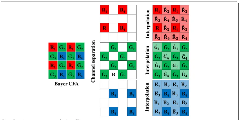
Among the various CFA patterns, the Bayer CFA pattern [26] is commonly used in digital cameras. It features B and R filters at alternating pixel locations in the horizon-tal and vertical directions, and G filters organized in a quincunx pattern at the remaining locations. Because each pixel has only one color sampled, a demosaicing al-gorithm must be employed to recover the empty infor-mation using a demosaicing process. There are four possible Bayer color filters as indicated in Fig. 1. Figure 1 presents the 2 × 2 Bayer pattern with its R, G, and B color filter elements, where two G elements are arranged in a diagonal setup and each R and B element fills the remaining space. In general, one of the four possible Bayer patterns can be used to capture the image under investigation. Let Cb(b= 1, 2, 3, 4) be a specific Bayer CFA configuration that is one of the four possible
con-figurations C1= [RGGB], C2= [GRBG], C3= [GBRG],
and C4= [BGGR]. The type of Bayer CFA pattern is
de-termined according to the order of the R pixel location (from left to right and from top to bottom) as indicated in Fig. 1.
and the inverse demosaiced signal with respect to all possible Bayer CFA configurations. The configuration that minimizes this cost function is selected as the spe-cific Bayer CFA pattern. The count of the intermediate values for various neighbor pixel patterns is defined as the cost function to identify the Bayer CFA pattern in [24]. This algorithm is based on the assumption that the majority of the interpolated values exist between the maximum and minimum values in the neighboring re-gion. Using the maximum counting value for each color channel, the specific Bayer CFA pattern is configured. However, the two conventional algorithms assume that the demosaiced image can be obtained based on a linear interpolation manner. The estimation error caused by these algorithms cannot be ignored for complex demo-saicing methods. We experimentally investigate that the assumption based on linear interpolation is not suitable for Bayer pattern identification.
For example, let us consider theC1Bayer pattern. In the RGGB Bayer pattern, demosaicing is an interpolation process used to estimatefR2;R3;R4;G1;G4;B1;B2;B3g
from the acquiredfR1;G2;G3;B4g. Figure 2 shows a
typ-ical demosaicing process. Because the kernel of the linear interpolator has the basic characteristics of a low-pass fil-ter, we assume that the variance of the original image block is greater that of the interpolated image block. To verify this assumption, we randomly extract 10,000 image blocks of size 256 × 256 from the Dresden image dataset [27] and calculate the probability that the variance of the original block is larger than that of the interpolated block. For this test, we exploit various demosaicing methods such as bilinear interpolation, adaptive homogeneity-directed (AHD) method [28], variable number of gradients (VNG) algorithm [29], aliasing minimization and zipper elimination (AMaZE) [30], DCB demosaicing [31], IGV demosaicing [32], linear minimum mean square error (LMMSE) demosaicing [33], and heterogeneity-projection hard-decision (HPHD) color interpolation [34].
Table 1 indicates the probabilities that the variance of the original block is larger than that of the interpolated
block in various interpolation methods. In this test, only four of the ten possible cases for the C1Bayer configur-ation are selected. For the bilinear interpolconfigur-ation, all probabilities are greater than 0.95 (bold numbers in Table 1). In this case, the probability itself is a reliable measure to estimate the Bayer CFA configuration. How-ever, we observe that the probabilities are significantly lower for the AMaZE, IGV, LMMSE, and HPHD demo-saicing methods. Therefore, the estimation of the CFA configuration based on the linear assumption is difficult to apply other than the demosaicing algorithm method, except for bilinear interpolation.
The conventional algorithms extract a fixed block at the center of the given image to estimate the Bayer CFA pattern configuration. Because an image is composed of backgrounds, edges, and textures, the fixed center block may have various types of image components depending on the given image. Therefore, the conventional methods could have an inefficient identification process because they use the same block regardless of the char-acteristics of the image. Furthermore, the background region can have a negative influence on estimating the Bayer pattern configuration because the characteristics of the background regions are similar to those of the ori-ginal pixel and the interpolated pixel. In this paper, we solve these problems by employing singular value decomposition.
3 Proposed Bayer CFA pattern identification method
Because the position of the R pixel is always diagonally opposite the position of the B pixel, the Bayer CFA pat-tern can be easily identified by only the position of the R or B channel. As indicated in Fig. 1, the four patterns are grouped by two categories according to the G
pos-ition, that is, [XGGX] and [GXXG], where X∈{R,B}.
step identification process. We first determine the diag-onal pair with R and B. Then, we estimate the position of R because the position of R directly determines the Bayer CFA pattern configuration.
3.1 Construction of color difference block
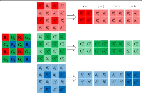
For a given color image I, letI(x,y) be the pixel value at the (x,y) position. We extract an image block Mof size M×M located at the center of the image. In this paper, we will omit the variables indicating position, such as x and y, as long as there is no confusion. Bold characters represent matrices, and non-bold italic characters imply scalar values. LetΑ∈{R,G,B} be a color component of
the cropped image block M. The color component can
be rearranged to four down-sampled blocks according to
the location of the pixels in the 2 × 2 Bayer pattern matrix as indicated in Fig. 1.Αcan be expressed as
Α¼ AmAð Þ1 1 AmA
2 ð Þ 2 AmA
3 ð Þ 3 AmA
4 ð Þ 4
h i
; ð1Þ
where ΑmΑi ð Þi is the down-sampled color component with size M/2 ×M/2, i∈{1, 2, 3, 4} is the location of the pixel in the 2 × 2 Bayer pattern matrix, andmA(i)∈{O,I}
is the indicator that represents whether the down-sampled block is interpolated or not, depending on its
position i at the Bayer CFA. In (1), O and I indicates
whether the block is original or interpolated, respect-ively. Figure 4 shows an example of color component decomposition for theC1Bayer pattern.
Table 1Probabilities that the variance of the original block is larger than that of the interpolated block for various demosaicing
algorithms (Bayer configurationC1is used) Demosaicing
method
Probabilities
Pr[σ2(R
1) >σ2( 4)] Pr½σ2ð ÞG2 >σ2ð ÞG1 Pr½σ2ð ÞG3 >σ2ð ÞG1 Pr½σ2ð ÞB4 >σ2ð ÞB1
Bilinear 0.9655 0.9512 0.9509 0.9596
AHD 0.4920 0.6865 0.7136 0.5236
VNG 0.7702 0.8749 0.8589 0.6934
AMaZE 0.5483 0.5345 0.5638 0.5843
DCB 0.8439 0.9588 0.9559 0.7331
IGV 0.5872 0.6816 0.6900 0.5794
LMMSE 0.5947 0.6600 0.6779 0.6623
HPHD 0.5139 0.4408 0.4538 0.5348
Average 0.6646 0.7235 0.7336 0.6588
Many demosaicing algorithms exploit spectral and spatial correlation for estimating empty pixels using neighboring pixels. Spectral correlation is based on the assumption that the color difference is virtually constant in a flat area. Spatial correlation means that the color values in a homogeneous image region are similar to
those in the neighboring regions. Therefore, the esti-mated missing color components are composed of the difference between the original sample and the filtered sample or between two interpolated samples in the ma-jority of the color interpolation algorithms. Based on this fact, we present a new CFA pattern identification algo-rithm using color difference image blocks.
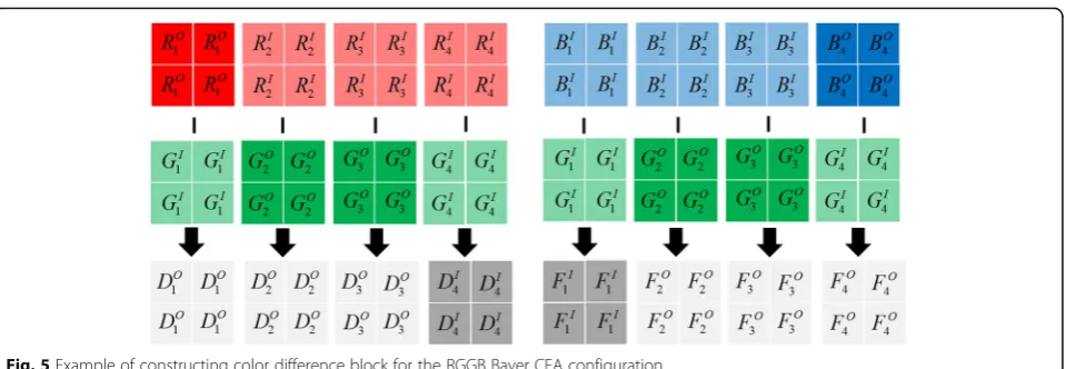
Let DmDi ð Þi be the color difference blocks between RmRð Þi
i andG mGð Þi
i . That is,
DmDð Þi
i ¼R mRð Þi
i −G mGð Þi
i ; ð2Þ
where mD(i)∈{O,I} is the indicator representing the
characteristics of the difference block DmDi ð Þi . In (2), mD(i) =O when (mR(i),mG(i)) = (O,I) or (mR(i),mG(i))
= (I,O);mD(i) =Iwhen (mR(i),mG(i)) = (I,I). In a similar
manner, letFmFi ð Þi be the color difference blocks between
BmBð Þi
i andGmG i ð Þ i .
FmFð Þi i ¼B
mBð Þi i −G
mGð Þi
i ; ð3Þ
wheremF(i)∈{O,I}. Figure 5 represents an example of
constructing a color difference block for the C1 Bayer
CFA configuration. As indicated in Fig. 5, two dark gray Fig. 3Two-step Bayer CFA pattern identification process
regions (DI
4 and FI1) consist of interpolated pixels; the
remaining six light gray areas consist of the difference between the original pixel and the interpolated pixel. The two difference blocks (DO
2 ¼RI2−GO2 and DO3 ¼RI3− GO
3) are composed of the original G pixels and the
inter-polated R pixels. It is assumed that the statistical charac-teristic of DO
2 and DO3 is similar. This will be the same
for FO2 and FO3. This fact is a clue to determining the R and B diagonal pair in the Bayer CFA pattern.
3.2 Identification process using singular values
Many demosaicing algorithms attempt to preserve or enhance edge components in the image. Therefore, various operations are performed in the edge compo-nents. For this reason, whereas the original edge and interpolated edge are easily distinguishable, it can be difficult to distinguish between the original and in-terpolated background areas. Hence, eliminating the background components in the image block can be useful for estimating the Bayer pattern configuration. Singular value decomposition can be one solution to remove the background components from the image block. The large singular values of an image block mainly contain low-frequency background informa-tion. Conversely, small singular values are associated with the high-frequency components of the block. They are likely to represent texture and edge re-gions. These characteristics of singular values have been applied to image compression [35, 36] and sali-ency detection [37] methods. In this paper, we at-tempt to remove large singular values to eliminate the background effect and present a CFA pattern
identification algorithm using the sum of the
remaining singular values.
The singular value decomposition of a square matrix J with size M/2 ×M/2 is the factorization of J into the product of three matrices as follows.
J¼UΣVT; ð4Þ
where U and V are orthogonal matrices andΣis an
di-agonal matrix with singular values on the didi-agonal.
There are M/2 singular values with the condition of
λ(1)≥λ(2)≥ ⋯ ≥λ(M/2)≥0, whereλ(n) is thenth singu-lar value. Let λDið Þn and λFið Þn be the nth singular
values forDmDi ð Þi andFmFi ð Þi, respectively. LetSDi and SFi
be the sums of the truncated λDið Þn and λFið Þn values
fromt(t> 0) toM/2, respectively. Then,SDi and SFi are
obtained by
SDi ¼
XM=2
n¼t
λDið Þn ; ð5Þ
SFi ¼
XM=2
n¼t
λFið Þn: ð6Þ
At this point, we defined(i) as the position facingi di-agonally. For example, ifi= 1, thend(i) = 4; ifi= 2, then d(i) = 3. The statistical characteristic of the two G com-ponents composing a diagonal pair are assumed to be similar. Therefore, the first purpose of the proposed
method is to determine a pair of more similar SDi and
SFi. If the pair of SD1 and SD4 is more similar than the
pair of SD2 and SD3, then SD1 and SD4 are assumed to
compose the diagonal pair of the two G components. This process is the same for SFi andSFd ið Þ. As a measure
for the similarity of each pair, we use the absolute differ-ence of the sum of truncated singular values.
Let VDkðk¼1;2Þ be the absolute difference between
SDi andSDd ið Þ. That is
VkD ¼SDk−SDd kð Þ: ð7Þ
In a similar manner, we defineVFk as the absolute
dif-ference betweenSFi andSFd ið Þas follows.
VFk ¼ SFk−SFd kð Þ
: ð8Þ
AmongVDk, we assume that having a larger difference
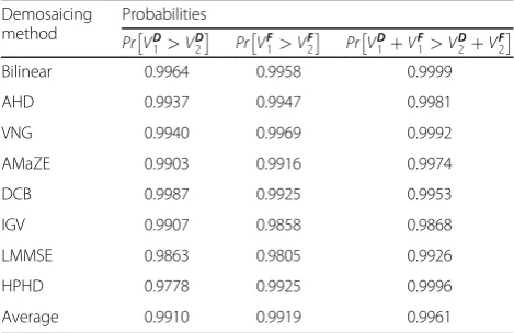
value forms a diagonal pair of R and B. This assumption is the same forVFk. To verify this assumption, we
calcu-late three probabilities of Pr VD1 >VD2
, Pr VF1 >VF2
, and Pr VD1 þVF1 >VD2 þVF2
for theC1CFA
configur-ation. We randomly selected 10,000 256 × 256 image blocks for this test. The other simulation conditions are the same as in Table 1. As illustrated in Table 2, the
average probabilities ranged from 0.9910 to 0.9961. Pr
VD1 þVF1 >VD2 þVF2
achieved the highest probability. From these facts, we can verify that the probabilities of VDk and VFk are useful measures for estimating the CFA
pattern configuration.
Let ~bð∈f1;2gÞ be the candidate index of the Bayer
CFA configuration. We obtain the kvalue with the
lar-gestVDk þVFk as the~b value. That is,
~
b¼ arg max
k V
D
k þVFk
: ð9Þ
From (9), we can determine the diagonal pair of R and B. For example, ifb~¼1, then the position of the R block will be 1 or 4. If b~¼2, then the R position will be 2 or 3. Consequently, the Bayer configuration indexb will be
~
b ord b~ . The next step is to determine the location of R. In the R-G blocks, the difference block having the ori-ginal R has higher frequency components than the dif-ference block having the interpolated R. Therefore, the singular value sum of the difference block having the original R will be larger than the difference block having the interpolated R. This fact is the same for the B and G blocks. Hence, we compareSDiþSFd ið Þ andSDd ið ÞþSFi to
estimate the Bayer CFA configuration. If SDiþSFd ið Þ
>SDd ið ÞþSFi, then the final CFA configuration will be
C~b; otherwise, the final CFA configuration will beCdð Þ~b .
That is,
b¼ ~b; ifSDiþSFd ið Þ >SDd ið ÞþSFid~b;otherwise
: ð10Þ
From (9) and (10), we can easily estimate the CFA pat-tern configuration.
3.3 Summary of proposed method
We first determine the size of the square image block to
identify the CFA pattern. We choose the image blockM
located at the center of the given image and decompose
the color component Α into four sub-blocks using (1).
For the decomposed color sub-blocks, we construct R minus G and B minus G difference blocks using (2) and (3), respectively. Then, the two sums of truncated singu-lar values are obtained using (5) and (6). The two abso-lute difference values are calculated using (7) and (8). The candidate index of the Bayer CFA configurationb~is estimated using (9). Finally, the Bayer CFA pattern index bis determined using (10). The overall algorithm for the proposed method is summarized in Table 3.
4 Simulation results and discussion 4.1 Test data sets and simulation conditions
We used 1460 raw images provided by the Dresden database [27] for our simulations. The camera types and detailed information regarding the test images are pre-sented in Table 4. We generated four Bayer CFA pat-terns for testing from the raw image data. For CFA interpolation, eight demosaicing algorithms including bi-linear interpolation, AHD method, VNG algorithm, AMaZE [29] method, DCB demosaicing, IGV
demosai-cing, LMMSE demosaicing, and HPHD color
interpolation were used in our experiments. CFA
inter-polations were performed using RawTherapee [32], a
Table 2Probabilities ofVD1 >VD2,VF1>VF2, andVD1þVF1>VD2
þVF2 for various demosaicing algorithms (Bayer configuration
C1is used) Demosaicing method
Probabilities
Pr V D1>VD2 Pr V F1>VF2 Pr V 1DþVF1>V2DþVF2
Bilinear 0.9964 0.9958 0.9999
AHD 0.9937 0.9947 0.9981
VNG 0.9940 0.9969 0.9992
AMaZE 0.9903 0.9916 0.9974
DCB 0.9987 0.9925 0.9953
IGV 0.9907 0.9858 0.9868
LMMSE 0.9863 0.9805 0.9926
HPHD 0.9778 0.9925 0.9996
Average 0.9910 0.9919 0.9961
Table 3Overall algorithm for proposed method
Input: A suspicious image.
Input parameters: Square block sizeMand truncated singular value pointt.
Output: Bayer CFA pattern configuration,Cb
1.Choose the image blockMlocated at the center of the given image.
2.For each color component, decompose the block into four sub-blocks using (1).
3.ComputeDimDð Þi andFimFð Þi using (2) and (3), respectively.
4.ComputeSmDð Þi D;i andS
mFð Þi
F;i using (5) and (6), respectively.
5.ComputeVDk andVFkusing (7) and (8), respectively.
6.Determine candidate indexb~using (9).
well-known cross-platform raw image-processing pro-gram. To identify the Bayer CFA pattern type, we tested the performance of the proposed algorithm for different block sizes including 512 × 512, 256 × 256, 128 × 128, 64 × 64, and 32 × 32. The cut point to obtain the trun-cated sum of singular values was set to t= (M/2)/2 in our simulations.
4.2 Comparisons of estimation performance
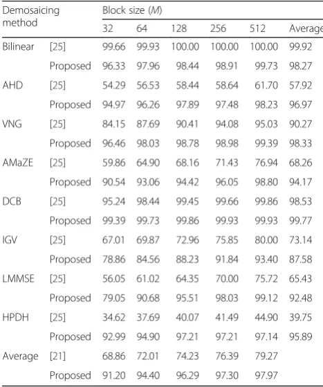
We compared the proposed method with the conven-tional method [25] in an environment without post-processing. Table 5 displays the Bayer CFA pattern iden-tification performance for the proposed method and conventional algorithm. The estimation accuracies for CFA pattern configuration were drawn from the eight demosaicing algorithms for different block sizes. The bold numbers in Table 5 indicate the highest identifica-tion performance. The average values in the horizontal direction represent the average for the demosaicing
method regardless of the block size. For all demosaicing algorithms except bilinear interpolation, the results of the proposed method are superior to those obtained using the conventional method. The conventional ap-proach has good identification performance for bilinear interpolation. This fact is because that the existing method basically exploits the characteristics of bilinear interpolation. However, the conventional method has poor detection rates for the more complex demosaicing methods that preserve or enhance high-frequency com-ponent of an image as shown in Table 5.
The proposed algorithm tries to achieve good identifi-cation performance for all demosaicing methods even with a slight performance degradation for bilinear inter-polating. In particular, the estimation accuracies of the proposed method demonstrate more than 92% for all demosaicing algorithms except the IGV interpolation method. The average values in the vertical direction in Table 5 indicate the average for the cropped block size regardless of the demosaicing algorithm. The estimation accuracy obtained by our identification method in-creased from 91.20 to 97.97% as the block size inin-creased. From Table 5, we observe that the estimation perform-ance for the CFA configuration increased as the block size increased.
We compared the computation time of the proposed and existing methods. All tests were performed on a desktop running 64-bit Windows 7 with 16.0 GB RAM and an Intel(R) Core(TM) i7-870 2.93 GHz CPU. For a 256 × 256 image block, the average CFA pattern identifi-cation time of the proposed method was approximately 0.035 s. The computation time of the conventional method for estimating the CFA configuration was ap-proximately 0.176 s. The proposed method was approxi-mately five times faster than the conventional approach.
4.3 Estimation performance with post-processing
We evaluated the proposed algorithm for different simu-lation conditions such as blurring, sharpening, and JPEG compression. For the blurring operation, we used a
Gaussian blur with five different parameters (σ=
0.50, 0.75, 1.00, 1.25, 1.50). The sharpened images were generated using a Laplacian operator with five different parameters (α= 0.1, 0. 2, 0.3, 0.4, 0.5). JPEG compressed
images were tested in our experiment (QF=
100, 90, 80, 75, 70). All tests were performed for a 256 × 256 block.
Table 6 displays the comparison between the existing algorithm and the proposed method with Gaussian blur for the different demosaicing methods. As indicated in Table 6, the proposed method is superior to the conven-tional method in terms of the average estimation per-formance according to both demosaicing algorithm and blur parameter. The average estimation accuracy of the
Table 4Camera models and image information in the
experiments
Camera model Number of images Image size
NIKON D200 728 3904 × 2616
NIKON D70 361 3040 × 2014
NIKON D70s 371 3040 × 2014
Table 5Estimation accuracy comparison between existing
algorithm and proposed method for various demosaicing methods (unit: %)
Demosaicing method
Block size (M)
32 64 128 256 512 Average
Bilinear [25] 99.66 99.93 100.00 100.00 100.00 99.92
Proposed 96.33 97.96 98.44 98.91 99.73 98.27
AHD [25] 54.29 56.53 58.44 58.64 61.70 57.92
Proposed 94.97 96.26 97.89 97.48 98.23 96.97
VNG [25] 84.15 87.69 90.41 94.08 95.03 90.27
Proposed 96.46 98.03 98.78 98.98 99.39 98.33
AMaZE [25] 59.86 64.90 68.16 71.43 76.94 68.26
Proposed 90.54 93.06 94.42 96.05 98.80 94.17
DCB [25] 95.24 98.44 99.45 99.66 99.86 98.53
Proposed 99.39 99.73 99.86 99.93 99.93 99.77
IGV [25] 67.01 69.87 72.96 75.85 80.00 73.14
Proposed 78.86 84.56 88.23 91.84 93.40 87.58
LMMSE [25] 56.05 61.02 64.35 70.00 75.72 65.43
Proposed 79.05 90.68 95.51 98.03 99.12 92.48
HPDH [25] 34.62 37.69 40.07 41.49 44.90 39.75
Proposed 92.99 94.90 97.21 97.21 97.14 95.89
Average [21] 68.86 72.01 74.23 76.39 79.27
proposed method ranged from 96.19 to 87.08% as the blurring effect increased. However, the estimation accur-acies for the bilinear interpolation case were significantly reduced. This is because the proposed algorithm uses primarily the high frequency components of the given block. In the case of the conventional method, we ob-serve that all the estimation results are degraded by per-forming the blurring operation. The estimation accuracy was significantly reduced when the blur parameter was greater than 0.75. Conversely, the average identification performance for bilinear interpolation was greater than the proposed method. In conclusion, the overall per-formance of the proposed scheme was superior to the existing algorithm and we achieved usable results when the blurring was applied.
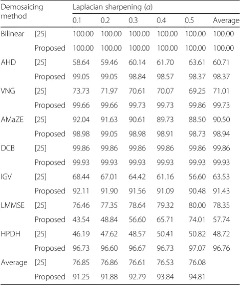
The estimation results for sharpening post-processing are displayed in Table 7. As indicated in Table 7, all esti-mation results demonstrate 100% for all bilinear interpolation cases. When sharpening operations are performed, the estimation accuracies of the proposed method increased for all demosaicing algorithms except the LMMSE interpolation method. In terms of block size, the estimation results generated by the proposed method were slightly reduced. This is because that the performance degradation has taken place considerably with the LMMSE demosaicing method. However, all the
average accuracies according to the different sharpening parameters are more than 91%. The estimation results using the existing method slightly increased by perform-ing a sharpenperform-ing operation. The conventional method that uses intermediate values to estimate the CFA con-figuration is based on the unchanging factor after
demo-saicing (background component). Because the
sharpening operation has less impact on the back-grounds and more on the high-frequency components, we can expect that there would be no performance change in the existing method. The overall average esti-mation performances of the proposed method remain high compared to the existing method for virtually all sharpening cases.
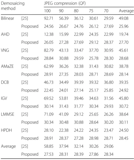
The CFA pattern identification results of performing various JPEG compressions are displayed in Table 8. As indicated in Table 8, the estimated performance of the proposed method is less than the conventional method in the majority of cases. Because the proposed method is based on truncated singular values, the increase in high frequency components due to the quantization error has a negative influence on the estimation of the Bayer pat-tern configuration. The average estimation accuracies of both methods are considerably low. Therefore, both al-gorithms are difficult to use in practical applications. Fu-ture studies on CFA pattern identification should
Table 6Estimation accuracy comparison between conventional
algorithm and proposed method with Gaussian blur for different demosaicing methods (unit: %). Block size fixed to 256 × 256
Demosaicing method
Gaussian blur (σ)
0.50 0.75 1.00 1.25 1.50 Average
Bilinear [25] 100.00 99.93 98.50 66.67 45.03 82.03
Proposed 91.97 68.64 53.81 46.12 42.72 60.65
AHD [25] 49.66 44.29 45.85 37.86 29.52 41.42
Proposed 97.21 96.80 96.67 96.19 95.92 96.56
VNG [25] 90.75 88.91 89.17 74.49 50.95 78.86
Proposed 99.05 99.12 98.44 98.10 97.48 98.44
AMaZE [25] 60.68 42.86 32.86 26.05 25.37 37. 56
Proposed 95.44 94.29 93.33 91.90 91.29 93.25
DCB [25] 98.64 92.45 81.02 48.10 33.81 70.80
Proposed 99.93 99.93 99.93 99.86 99.73 99.88
IGV [25] 69.18 46.26 18.37 12.65 10.41 31.06
Proposed 90.75 87.55 84.29 81.70 80.20 84.90
LMMSE [25] 53.81 26.19 12.65 10.48 13.95 23.42
Proposed 98.10 97.62 96.94 96.39 94.56 96.72
HPDH [25] 40.00 33.06 28.64 21.63 20.61 28.79
Proposed 97.07 96.53 95.71 95.17 94.76 93.25
Average [25] 70.34 59.24 50.88 37.03 28.71
Proposed 96.19 92.56 89.89 88.18 87.08
Table 7Estimation accuracy comparison between conventional
algorithm and proposed method with Laplacian sharpening for different demosaicing methods (unit %). Block size fixed to 256 × 256
Demosaicing method
Laplacian sharpening (α)
0.1 0.2 0.3 0.4 0.5 Average
Bilinear [25] 100.00 100.00 100.00 100.00 100.00 100.00
Proposed 100.00 100.00 100.00 100.00 100.00 100.00
AHD [25] 58.64 59.46 60.14 61.70 63.61 60.71
Proposed 99.05 99.05 98.84 98.57 98.37 98.37
VNG [25] 73.73 71.97 70.61 70.07 69.25 71.01
Proposed 99.66 99.66 99.73 99.73 99.86 99.73
AMaZE [25] 92.04 91.63 90.61 89.73 88.50 90.50
Proposed 98.98 99.05 98.98 98.91 98.73 98.94
DCB [25] 99.86 99.86 99.86 99.86 99.86 99.86
Proposed 99.93 99.93 99.93 99.93 99.93 99.93
IGV [25] 68.44 67.01 64.42 61.16 56.60 63.53
Proposed 92.11 91.90 91.56 91.09 90.48 91.43
LMMSE [25] 76.46 77.35 78.64 79.32 80.00 78.35
Proposed 43.54 48.84 56.60 65.71 74.01 57.74
HPDH [25] 46.19 47.62 48.57 50.41 50.82 48.72
Proposed 96.73 96.60 96.67 96.73 97.07 96.76
Average [25] 76.85 76.86 76.61 76.53 76.08
proceed toward increasing the estimation performance, even in the JPEG compression environment.
4.4 Discussion
The proposed method has a fairly high accuracy in de-termining the Bayer CFA pattern type. Our method can be used as the first step of the image forensic applica-tions using the CFA pattern distortion. The results of the proposed method are superior to those obtained using the conventional method for all demosaicing algo-rithms except bilinear interpolation. However, the pro-posed algorithm as well as the conventional methods cannot be practically applied to a JPEG compressed image. The future challenge will be to increase the estimation.
5 Conclusions
We presented an efficient CFA pattern identification in this paper. We constructed a color difference image to reflect the characteristics of different demosaicing methods. To estimate the CFA pattern configuration, we exploited singular value decomposition. The truncated sum of the singular values was used to identify the Bayer CFA pattern. Experimental results confirmed that the proposed method generated acceptable estimation re-sults in identifying the pattern. Compared with the
conventional method, the proposed method worked well except for bilinear interpolation and JPEG compression.
Funding
This research was supported by the Basic Science Research Program through the National Research Foundation of Korea (NRF) funded by the Ministry of Education, Science, and Technology (NRF-2015R1D1A3A01019561).
Authors’contributions
JJ Jeon and JJ Shin proposed the framework of this work, carried out the whole experiments, and drafted the manuscript. IK Eom initiated the main algorithm of this work, supervised the whole work, and wrote the final manuscript. All authors read and approved the final manuscript.
Competing interests
The authors declare that they have no competing interests.
Publisher’s Note
Springer Nature remains neutral with regard to jurisdictional claims in published maps and institutional affiliations.
Received: 13 April 2017 Accepted: 4 July 2017
References
1. H Farid, A survey of image forgery detection. IEEE Signal Process. Mag.
2(26), 16–25 (2009)
2. B Mahdian, S Saic, A bibliography on blind methods for identifying image forgery. Signal Process. Image Commun.25(6), 389–399 (2010)
3. Z He, W Lu, W Sun, J Huang, Digital image splicing detection based on Markov features in DCT and DWT domain. Pattern Recog.45(12), 4292–4299 (2012) 4. X Zhao, S Wang, S Li, J Li, Passive image-splicing detection by a 2-D
noncausal Markov model. IEEE Trans. Circuits Syst. Video Technol.25(2), 185–199 (2015)
5. M El-Alfy, MA Qureshi, Combining spatial and DCT based Markov features for enhanced blind detection of image splicing. Pattern Anal. Appl.18(3), 713–723 (2015)
6. JG Han, TH Park, YH Moon, IK Eom, Efficient Markov feature extraction method for image splicing detection using maximization and threshold expansion. J. Electron. Imaging.25(2), 023031 (2016)
7. K Bahrami, AC Kot, L Li, H Li, Blurred image splicing localization by exposing blur type inconsistency. IEEE Trans. Inf. Forensics Security10(5), 999–1009 (2015) 8. DM Uliyan, HA Jalab, AW Wahab, P Shivakumara, D Sadeghi, A novel forged
blurred region detection system for image forensic applications. Expert Syst. Appl.64, 1–10 (2016)
9. H Yao, S Wang, X Zhang, C Qin, J Wang, Detecting image splicing based on noise level inconsistency. Multimed. Tools Appl.75(10), 12457–79 (2017) 10. S Lyu, X Pan, X Zhang, Exposing region splicing forgeries with blind local
noise estimation. Int. J. Comput. Vis.110(2), 202–221 (2014)
11. Z Lin, J He, X Tang, CK Tang, Fast, automatic and fine-grained tampered JPEG image detection via DCT coefficient analysis. Pattern Recog.42(11), 2492–2501 (2009)
12. T Bianchi, A Piva, Image forgery localization via block-grained analysis of JPEG artifacts. IEEE Trans. Inf. Forensics Secur.7(3), 1003–1017 (2012) 13. G Chierchia, G Poggi, C Sansone, L Verdoliva, A Bayesian-MRF approach for
PRNU-based image forgery detection. IEEE Trans. Inf. Forensics Secur.9(4), 554–567 (2014)
14. P Korus, J Huang, Multi-scale analysis strategies in PRNU-based tampering localization. IEEE Trans. Inf. Forensics Secur.12(4), 809–824 (2017) 15. WC Hu, WH Chen, DY Huang, CY Yang, Effective image forgery detection of
tampered foreground or background image based on image watermarking and alpha mattes. Multimed. Tools Appl.75(6), 3495–3516 (2017) 16. O Benrhouma, H Hermassi, A El-Latif, S Belghith, Chaotic watermark for
blind forgery detection in images. Multimed. Tools Appl.75(14), 8695–8718 (2016)
17. P Ferrara, T Bianchi, A De Rosa, A Piva, Image forgery localization via fine-grained analysis of CFA artifacts. IEEE Trans. Inf. Forensics Secur.7(5), 1566– 1577 (2012)
18. H Cao, AC Kot, Accurate detection of demosaicing regularity for digital image forensics. IEEE Trans. Inf. Forensics Secur.4(4), 899–910 (2009)
Table 8Estimation accuracy comparison between conventional
algorithm and proposed method with JPEG compression for different demosaicing methods (unit %). Block size fixed to 256 × 256
Demosaicing method
JPEG compression (QF)
100 90 80 75 70 Average
Bilinear [25] 92.71 56.39 36.12 30.61 29.59 49.08
Proposed 24.56 26.67 24.76 26.12 27.69 25.96
AHD [25] 12.38 15.99 22.99 24.35 22.99 19.74
Proposed 26.05 27.28 27.69 29.12 28.37 27.70
VNG [25] 82.79 43.13 33.47 37.70 30.95 45.61
Proposed 28.84 30.88 29.59 25.78 28.30 28.68
AMaZE [25] 62.99 36.26 32.38 31.43 30.82 38.78
Proposed 28.91 27.35 28.03 28.71 28.69 28.14
DCB [25] 46.73 34.49 39.39 39.32 36.80 39.35
Proposed 22.45 24.01 27.14 25.17 25.85 24.92
IGV [25] 69.52 53.81 39.46 34.63 31.56 45.80
Proposed 30.14 31.43 31.77 30.34 29.93 30.72
LMMSE [25] 71.09 41.09 29.12 25.65 26.26 38.64
Proposed 30.34 30.48 30.88 28.64 30.20 30.11
HPDH [25] 28.10 22.38 24.22 24.35 23.47 24.50
Proposed 28.91 28.37 27.28 28.98 28.71 28.45
Average [25] 58.85 37.94 32.14 30.26 29.06
19. S Bayram, HT Sencar, N Memon, Classification of digital camera-models based on demosaicing artifacts. Digit. Invest.5, 49–59 (2008)
20. CH Choi, HY Lee, HK Lee, Estimation of color modification in digital images by CFA pattern changes. Forensic Sci. Int.226, 94–105 (2013)
21. Y Huang, Y Long,Demosaicking recognition with applications in digital photo authentication based on a quadratic pixel correlation model. Proceedings of the 2008 IEEE Conference on Computer Vision and Pattern Recognition, 2008, pp. 1–8
22. AC Gallagher, TH Chen,Image authentication by detecting traces of demosaicing. Proceedings of IEEE Computer Society Conference on Computer Vision and Pattern Recognition Workshops, 2008, pp. 1–8 23. YH Huang, KL Chung, TJ Lin, Efficient identification of arbitrary color filter
array images based on the frequency domain approach. Signal Process.
115, 20–129 (2015)
24. M Kirchner,Efficient estimation of CFA pattern configuration in digital camera images. Proceedings of SPIE Media Forensics and Security II, vol. 7541, 2010, p. 754111
25. CH Choi, JH Choi, HK Lee,CFA pattern identification of digital cameras using intermediate value counting. Proceedings of ACM Workshop in Multimedia and Security, 2011, pp. 21–26
26. BE Bayer, U.S. Patent No. 3,971,065. (U.S. Patent and Trademark Office, Washington, DC, 1976), https://www.google.com/patents/US3971065. 27. T Gloe, R Bohme,The‘Dresden Image Database’for benchmarking digital
image forensics. Proceedings of the 25th Symposium on Applied Computing, 2010, pp. 1585–1591
28. K Hirakawa, TW Parks, Adaptive homogeneity directed demosaicing algorithm. IEEE Trans. Image Process.14(3), 360–369 (2005)
29. E Chang, S Cheung, DY Pan,Color filter array recovery using a threshold-based variable number of gradients. Proceedings of SPIE, Sensors, Cameras, and Applications for Digital Photography, 1999, pp. 36–43
30. E Martinec, P Lee, AMAZE demosaicing algorithm. http://www.rawtherapee. com/. Accessed 14 Nov 2016
31. J Gozd, DCB demosaicing algorithm. http://www.linuxphoto.org/html/dcb. html. Accessed 14 Nov 2016
32. G Horvath, http://www.rawtherapee.com/. Accessed 27 Mar 2017 33. L Zhang, X Wu, Color demosaicking via directional linear minimum mean
square-error estimation. IEEE Trans. Image Process.14(12), 2167–2178 (2005) 34. CY Tsai, KT Song, Heterogeneity-projection hard-decision color interpolation using spectral-spatial correlation. IEEE Trans. Image Process.16(11), 78–91 (2007)
35. AM Rufai, G Anbarjafan, H Demirel, Lossy image compression using singular value decomposition and wavelet difference reduction. Digit Signal Process.
24, 117–123 (2014)
36. A Ranade, SS Mahabalarao, S Kale, A variation on SVD based image compression. Image Vis. Comput.25(6), 771–777 (2007)