R E S E A R C H A R T I C L E
Open Access
Demand response visualization tool for electric
power systems
Michael Negnevitsky
*and Koon Wong
Abstract
Background:Demand response (DR) is referred to programs designed to manage and control electric loads. DR represents one of the vital tools utilized in power distribution networks to improve network efficiency. Effective implementation of DR programs delivers operational benefits such as reduced peak demands and relieved overloads, which are essential in a power system with growing penetration of fundamentally intermittent renewable energy sources.
Methods:This paper presents a visualization tool for optimising DR programs for domestic hot water systems in distribution power networks. The tool accurately models and predicts potential peak demand reductions through direct load control of domestic hot water systems. It employs a multi-layer thermally stratified hot water cylinder model and Monte Carlo simulations to generate hot water load profiles of domestic customers. To meet peak reduction targets set by the tool user, switching programs found via iterative optimizations are applied to hot water systems.
Results:The structure and individual components of the tool are described, and case studies are presented. Impacts of different switching programs on customer’s comfort are evaluated and discussed.
Conclusion:The visualization tool is designed to recommend optimum DR switching programs for domestic water heating systems. The tool can assess the performance of a DR switching program by estimating potential peak load reductions and customer comfort characterized by the probability of cold showers. A power system operator can use this tool to determine the available domestic water heating load in a controlled area, and predict the potential reduction in peak load.
Keywords:Visualization tool; Demand response; Smart grid; Electric power system
Background
Electric power systems are undergoing a profound change. This change is driven by several factors that in-clude technical, economic and environmental factors. We need to deal with an aging infrastructure of power systems and maintain the required level of grid reliabil-ity. We need to integrate renewable energy sources, par-ticularly wind and solar, and provide secure power supply to our customers, and at the same time improve operational efficiency. The emerging changes and chal-lenges are particularly significant for distribution grids, where the level of automation or“smartness”is relatively low. Manual and“blind”operations along with old elec-tromechanical relays are to be transformed into a“smart
grid”. This transformation is necessary to meet environ-mental targets, accommodate distributed generation, and support plug-in electric vehicles. In fact, these needs present the power industry with the biggest challenge it has ever faced. On one hand, the transition to the“grid of the future” has to be evolutionary– we still need to supply electricity to our customers to keep the lights on. On the other hand, the challenges associated with the smart grid are significant enough to expect revolutionary changes in power system design and operation.
In the past, power utilities aimed to accurately forecast consumer demand for electricity, and then planed the growth of the power supply accordingly. But the energy crisis in the 1970s interfered in this process. In the 1970s the economies of the major industrial countries, particularly the United States, Canada, Western Europe, * Correspondence:[email protected]
School of Engineering and ICT, University of Tasmania, Tasmania, Australia
Japan, Australia, and New Zealand were heavily affected and faced substantial petroleum shortages. As a result, predictable demand and low-cost supply, the founda-tions of traditional planning, became harder and harder to achieve (Wayne and Gellings, 1984). It was the time for power companies to turn their attention to the de-mand side.
Demand response (DR) was introduced more than 30 years ago for shifting or reducing peak electricity de-mand (Strbac, 2008). Power systems have been built to meet peak demand–the maximum demand dictates the size of generators and ratings of transmission lines and transformers even if peaks last just a few hours per year. Billions have been spent on extra capacity and infrastruc-ture to cater for these few hours. On the other hand, power utilities could avoid costly investments by shifting or reducing peak demand. Thus, it made perfect sense to offer lower“interruptible”or“curtailable”rates to large in-dustrial and commercial customers for the right to tem-porarily reduce their electricity consumption.
With the push for energy conservation, DR is becom-ing a vital tool under the broad smart grid paradigm. This paper outlines some experience obtained at Univer-sity of Tasmania, Australia in the development and im-plementation of a visualisation tool for estimating impacts of demand response programs on loading of power transformers and transmission lines in electric grid. Section The concept of demand response in electric power systems provides a definition of DR and discusses its benefits for power utilities and electricity consumers. Section Methods describes the development of the RD visualisation tool for domestic water heating systems, and Section Results and discussion presents results of the tool implementation.
The concept of demand response in electric power systems
Demand response implies many activities such as direct load control, peak shaving, peak shifting, and various
load management strategies. According to the US Fed-eral Energy Regulatory Commission, DR is defined as:
“Changes in electric usage by end-use customers from their normal consumption patterns in response to changes in the price of electricity over time, or to in-centive payments designed to induce lower electricity use at times of high wholesale market prices or when system reliability is jeopardized”.
Effective implementation of DR programs delivers op-erational benefits such as reduced peak demands and re-lieved overloads, which are essential in a power system with growing penetration of fundamentally intermittent renewable energy sources (Strbac, 2008). Successful DR programs also provide economic gains such as deferrals of costly network upgrades as well as network security enhancements. Moreover, in a deregulated electricity market, DR programs offer opportunities for aggregation of demand reduction to support market and network op-erations of a power system (Nguyen et al. 2011). In addition, consumers receive financial incentives through participation in DR programs.
The fundamental benefit offered by demand response is flexibility. In power systems, flexibility is necessary to address critical situations and contingencies when they occur. Today, flexibility is mostly provided by conven-tional generators because renewable energy sources have very limited capacity to deliver flexibility to the power system. Demand response can provide additional flexi-bility from the demand side. And it is not always about disconnecting loads. Flexibility also means increasing de-mand when there is surplus energy and the electricity price is very low or even negative. In general, demand response promotes efficient pricing and efficient utilisa-tion of resources.
However, before we consider all potential benefits of demand response, a word of caution. Flexibility on the demand side has to compete with flexibility offered by
new generation technologies, grid investments and en-ergy storage solutions. Demand response still needs to overcome market rules, regulatory issues, consumer haviour, and technology and infrastructure barriers be-fore it can reach its real potentials. In the long run, however, investments in generation, consumption and grid may all be just alternative ways to address the need for flexibility in a sustainable energy system of the future.
So, what are benefits provided by demand response? They can be found in the improved economic efficiency of electricity markets, increased reliability of power sup-ply, financial benefits received by electricity consumers and enhanced sustainability of power systems. All these benefits are related to the flexibility offered on the de-mand side.
Economic benefits are associated with the ability of de-mand response to defer and even avoid new capital in-vestments in infrastructure (both in generation and grid) by flattening the demand curve. Demand response can also displace the most expensive peak generators. All this leads to lowering wholesale market prices and im-proving efficiency of the electricity market. Consumers participating in demand response programs also receive financial benefits in the form of the bill savings and in-centive payments.
Reliability benefits are associated with changes in elec-tricity usage, which enable power utilities to meet peak loads, and avoid blackouts when there is not enough generation to satisfy demand. In addition, demand re-sponse can provide ancillary services such as contin-gency reserves, regulation and load following. Demand
Figure 2The average number of showers versus family size.
response can react in under a second or within minutes, depending on the type of ancillary service required.
Environmental benefits are provided by enabling power utilities to avoid the use of peaking power plants or“ pea-kers”. Peakers typically have higher greenhouse gas emis-sions. However, most important environmental benefits can be achieved via a large-scale integration of renewable resources such as wind and solar. Because demand response can act as a form of energy storage, it can facilitate in managing periods of excessive generation through the provision of load-following and regula-tion services that can both increase or decrease demand.
There are three different methods to implement DR in a power distribution network. In indirect load control, consumers manually adjust their consumption in re-sponse to incentive programs such as time-of-use (TOU) tariffs (Heussen et al. 2012). In autonomous load control, devices autonomously adjust their consumption in response to detected changes in the power system or to commands sent from the control centre. In direct load control (DLC), devices are centrally controlled by the utility operator (Kondoh, 2011).
Water heating load forms a significant share of the total domestic demand. For example, Elphick (2009) es-timated that water heating load accounts for up to 40% of domestic energy consumption in Australia, and around one third in Tasmania, Australia. Moreover, do-mestic water heating systems represent insulated ther-mal energy storages that continually supply hot water even during periods of power interruption. Hence, they are commonly targeted for DR programs to reduce peak loads and improve the load factor. Well-designed DR programs minimize customer discomfort due to cold showers.
Many schemes for DLC of domestic hot water systems have been proposed. A practical approach introduced in McKelvie et al. (1992) uses a ripple injection system to issue switching signals to households grouped under dif-ferent modulation codes. Studies in Nehrir et al. (2007) focused on voltage control to reduce domestic hot water loads. In Gomes et al. (1999), hot water load profiles were simulated using physical models of domestic loads. Households were grouped by the family size to study the effect of DR switching programs on peak load reduction and customer comfort level. In van Tonder and Lane
Figure 4The probability distribution of the shower starting time.
(1996), peak load reduction was studied by considering the number of switching groups, target value and a sin-gle time-triggered control. In Gomes et al. (2004), evolu-tionary algorithms formed the basis for optimizing DR switching programs while maintaining customer satis-faction. A smart grid based control algorithm perform-ing DR on a modified domestic hot water system was proposed by Kondoh et al. (2011) to regulate the ag-gregated power consumption. Linear programming was used by Lee and Wilkins (1983) to find optimal DR strategies.
The next section presents the development of a visual-isation tool that assists in designing a DR program to de-liver desired peak load reductions while maintaining satisfactory level of comfort for all customers. The tool estimates the available domestic water heating loads in a controlled area, determines optimal switching pro-grams and presents results to the user in a graphical form. A switching program refers to a direct load con-trol schedule applied to domestic water heating sys-tems (to strategically switch them on and off ) in order to achieve a desired load reduction during peak periods.
Methods
General structure of the DR visualization tool
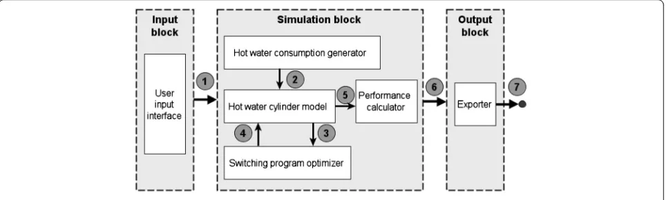
Main modules of the tool are shown in Figure 1, as dem-onstrated in Negnevitsky and Wong (2015). The modules are grouped in three main functional blocks. The num-bered grey circles represent inputs and outputs (I/O).
The Input block represents the user interface, which allows the tool user to enter parameters required for simulation (the number of households in the controlled area, the number of Monte Carlo simulations, the de-sired peak reduction, etc.) as well as to view default pa-rameters and change them if necessary. The Simulation block is the main block of the tool; it contains four
modules: the hot water consumption generator, hot water cylinder model, switching program optimizer, and performance calculator. The Output block contains the exporter, which exports the data to an external (Excel) file.
Default parameters and parameters entered by the user via the user input interface are represented by I/O 1. The hot water consumption generator receives I/O 1 and de-termines hot water consumption profiles for individual households; these profiles are represented by I/O 2. The hot water cylinder model receives I/O 2 and calculates un-controlled water heating loads and shower temperatures for the households; the results are represented by I/O 3. The user can observe the aggregate uncontrolled load curve of the households in the controlled area, and proceed with the optimization of switching programs. The switching program optimizer receives I/O 3 and produces switching programs based on the user-defined parameters (the desired peak reduction target, control periods etc.). The best switching programs are presented to the user, so that he/she can select the most suitable switching program. The hot water cylinder model then calculates controlled water heating loads (I/O 5) by applying the user-selected switching program (I/O 4) to the hot water consumption profiles (I/O 2). The performance calculator receives I/O 5 and determines key performance indicators such as peak reductions and customer’s comfort. Results in the form of 24-hour load curves are presented to the user (I/O 6), and exported to an external file (I/O 7) via the exporter.
Table 1 Family types and their distributions
Family type 1 2 3 4
Family size Very small Small Average Large
Number of residents 1 2 to 3 4 to 5 6 and above
Distribution in a population 25% 50% 22.5% 2.5%
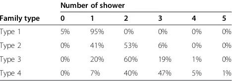
Table 2 Shower probabilities for different families
Number of shower
Family type 0 1 2 3 4 5
Type 1 5% 95% 0% 0% 0% 0%
Type 2 0% 41% 53% 6% 0% 0%
Type 3 0% 20% 60% 19% 1% 0%
Type 4 0% 7% 40% 47% 5% 1%
Table 3 Shower lengths and gaps between showers
Parameter Min
(min)
Max (min)
Mean (min)
Standard deviation (min)
Shower length 5 15 8 4
Shower gap 5 7 6 1
Hot water consumption generator
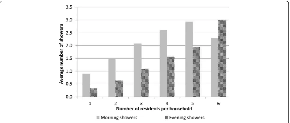
The first step in the development of the hot water con-sumption generator was to acquire knowledge of hot water consumption patterns of households in the controlled area. To achieve this objective, a telephone survey was con-ducted on 1000 randomly selected households across Tas-mania. It recorded demographic data (e.g. number of usual residents, combined income etc.) and details of hot water usages (e.g. average number of showers per day, average shower length etc.) of the surveyed households. This sur-vey focused on two peak periods in the Tasmanian power distribution network, i.e. morning and evening peaks from 6 am to 10 am and from 5 pm to 8 pm, respect-ively. Figures 2 and 3 show major results of the sur-vey. Figure 2 suggests a positive correlation between the average number of showers and the family size, in the morning and evening peaks. An unexpected drop in the average number of morning showers in house-holds with six or more residents can be explained by a relatively small sample size of this household type (just 2.3% of the total surveyed households).
As can be seen in Figure 3, the length of a shower can vary from 2 min to 15 min, however, a great majority of showers (about 51%) last from 5 min to 8 min.
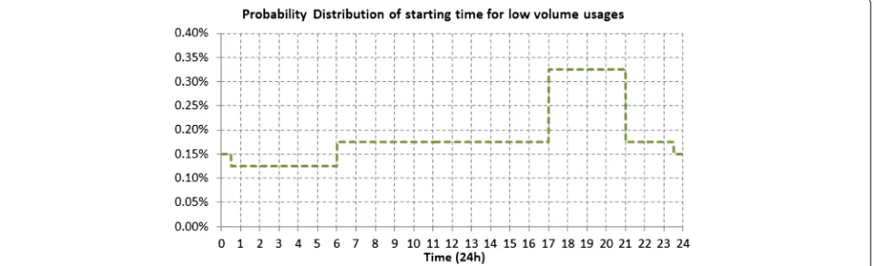
To estimate domestic hot water consumption pro-files, we also acquired energy metering data of 279 households across Tasmania. These data were obtained from meters dedicated for metering electric water heating alone, and represented water heating energy consumption of individual households recorded in 5-minute intervals. We considered two types of hot water usages: high volume usage that lasts for more than 5 min and low volume usage that lasts for 5 min or less. Based on the modelling, 1 min of hot water usage requires approximately 10 min of heating to re-store the temperature set by the thermostat. Thus, a continuous energy consumption (a switched-on condi-tion of the electric water heater) for a period of more than 50 min is regarded as a high volume usage (rep-resented by showers), and a consumption of less than or equal to 50 min is regarded as a low volume usage. Using weekday data only, we derived probability distributions of
Figure 7Measured and predicted power consumptions, normalized to 2400 (W).
the starting time for showers (Figure 4) and low volume us-ages (Figure 5).
Both surveys and energy metering data revealed that do-mestic hot water consumption depends mostly on the fam-ily size. Therefore, all households in a controlled area are divided into four groups according to the family type based on the number of residents in a household. Table 1 shows a typical distribution of families in a controlled area.
We need also specify probabilities of household occupants taking morning showers only, evening showers only, or both. Demographic data (Australian Bureau of Statistics, 2012), and household energy consumption records are used to esti-mate probabilities in Table 2, which determine the number of showers each family type take in the morning, evening, or morning and evening. Similar to showers, the probability of a low volume usage depends on the family size of a house-hold. The tool uses multipliers to scale this probability up based on the family type. Default values of the multipliers are 1.0, 1.2, 1.6 and 2.0, respectively. The tool user can redefine these values, if required. Figure 5 gives the probability of a low volume usage occurring in a household at a given time.
Shower lengths and gaps between consecutive showers are specified by their mean, maximum and minimum values. We define minimum and maximum to discard unrealistic values (e.g., a one-minute shower) in prob-abilistic simulations. Normal distributions are assumed. Default values used by the tool are shown in Table 3. A
low volume usage is denoted as a single 5-min draw. If required, the user can redefine these values.
The starting time of each hot water usage is specified based on probability distributions derived from actual energy metering data.
The tool employs a Monte Carlo approach to generate hot water consumption profiles for each household. First, the tool generates random values to determine specific parame-ters for a single household: family type, when showers are taken (morning, or evening, or morning and evening), num-ber of showers, numnum-ber of low volume usages, length of each shower and each gap between consecutive showers, starting time for each shower and each low volume usage. Next, using these parameters, the tool generates a 24-hour hot water consumption profile for a single household. The tool then repeats the profile generation process for a specified number of households using a new set of random values each time. Finally, the whole process is repeated for the re-quired number of Monte Carlo iterations. Based on the gen-erated hot water profiles, we can now proceed with calculating loads associated with household hot water usages. However, we need to develop a hot water cylinder model first.
Hot water cylinder model
The block diagram of the system with a single heating element is shown in Figure 6. For predicting the shower
Figure 9Measured and predicted shower temperatures in a shower schedule.
temperature and power consumption for domestic water heating systems accurately, we develop a hot water cylin-der model based on the most common domestic water heating system in Tasmania, which has a 165 L cylin-drical storage tank and a single 2.4 kW heating element. We validated the model with experimental data and found that predicted and measured values were closely matched. The measured and predicted values of normal-ized power consumption and top layer temperature over 48 hours are shown in Figures 7 and 8. Figure 9 shows the measured and predicted shower temperatures during four successive showers.
We found that the mean prediction error in the total energy consumption was less than 6%, while the mean absolute error in predicted shower temperature was less than 3°C. It was considered acceptable for the model to be used in the tool.
Performance calculator
The performance calculator has two main functions: cal-culating peak reductions in the water heating load and estimating the customers comfort level.
First, it determines an average uncontrolled load profile for each household. The average uncontrolled load profile for a household represents an average profile of the household ob-tained over a specified number of Monte Carlo iterations.
Then, it determines an aggregate uncontrolled load curve LU by aggregating uncontrolled load profiles for all households. An aggregate controlled load curveLCis obtained in a similar manner after a switching program is applied to the uncontrolled loads produced by the hot water cylinder model for individual households. The peak load reductionRτof the control periodτis defined as
Rτ¼1−max L½ Cð Þτ
max L½ Uð Þτ ð
1Þ
where max[LC(τ)] and max[LU(τ)] are the peaks of LC andLUthe control periodτ, respectively.
The customer’s comfort level depends on the frequency (or probability) of getting a “cold shower”— the event when the shower temperature drops below the comfort temperature (e.g. 43°C) specified by the tool user. Pre-ferred shower temperatures range from 40°C to 44°C, Ohnaka (1994). Because of a large number of households in the controlled area, we can assume the same comfort temperature for all customers. The tool allows the user to change the comfort temperature if required.
Switching program optimization
Figure 10 shows a block diagram of the switching program optimizer. Here I/Os are depicted as numbered blocks. I/O 1 represents parameters of the control management sys-tem, I/O 2 optimization parameters, I/O 3 uncontrolled loads generated by the hot water cylinder model, and I/O 4 represents optimized switching programs.
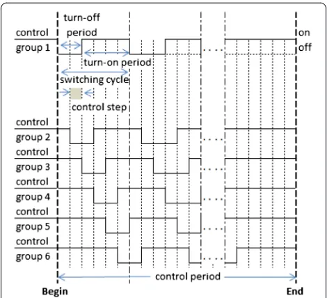
The switching program generator uses user-specified control management system parameters and optimized turn-off periods from the optimizer to create switching pro-grams, as shown in Figure 11. Here a control step is the smallest switching time interval, and a turn-off period is the time interval where the water heating system is turned off for a number of consecutive control steps. A switching cycle consists of the turn-off period followed by the turn-on period. A control period consists of multiple switching
Figure 11A switching program and its control management system parameters.
cycles (there are two control periods – for the morning peak and for the evening peak). Control groups are formed by shifting the switching cycles by one or more control steps. To ensure the time-shifted switching cycles are con-tained within a control period, each control group has one switching cycle less than the control period. In Wong and Negnevitsky (2013), it was demonstrated that division of households based on the family type does not significantly affect the comfort level of household residents. Therefore, the entire set of households can be divided into control groups of approximately the same size regardless of the family type of a household.
The load estimator determines the total controlled water heating load by applying a switching program to uncon-trolled loads of individual households. The load estimator sets the load to zero during the turn-off periods of the ap-plied switching program and restores the load during the turn-on periods. Water temperature is not considered in the load estimation.
The main function of the optimizer is to optimize turn-off periods of a switching program. It consists of the user-defined control period (UDCP) optimizer and the optimized control period (OCP) optimizer.
The UDCP optimizer determines turn-off periods based on the user-defined control periods and the peak load reduc-tion targets. The control periods remain unchanged throughout the optimization process. The UDCP optimizer implements an iterative process to minimize the mean error between the user-defined targetLTand the estimated aggre-gate controlled loadLCin each switching cycle of a switching program. To calculate required changes in the turn-off period for each switching cycle, it applies proportional and integral (PI) functions to the errors. In Figure 12, e(j,k)and
τoff(j,k) are the mean error and the turn-off period of switch-ing cyclejin iterationk, respectively;Kpis the proportional gain andTithe integral time of the PI functions.
The proportional function multiplies the error by Kp. The integral function sums the errors of switching cycle
Figure 13Initial control period in relation to LT and LU.
j from the previous (S-1) iterations to the current one, and multiplies the result by Kp/Ti. The sum of the current turn-off period and outputs from PI functions is converted by the limiter function into an integer be-tween the minimum and maximum values. The final re-sult is the turn-off period for the next iteration.
The OCP optimizer determines turn-off periods and con-trol periods of a switching program based on the user-defined peak load reduction targetLT. First, it finds the start-ing timetsand finishing timetfof the initial control period. The timetsis found as the first intersection of the aggregate uncontrolled loadLUand the targetLT, as shown in Figure 13. To avoid a high payback peak after the control period, the finishing timetfis found by solving the following equation:
Z tf
ts
LUð Þt ⋅dt¼LT⋅tf−ts ð2Þ
where the left hand term represents the total uncon-trolled energy consumption betweentsandtf.
To further minimize the error betweenLC and LT, the OCP optimizer iteratively tunes the switching program optimized by the UDCP optimizer. The OCP optimizer increases or decreases the turn-off period τoff of each switching cycle to minimize the error between LT and
LC. We define three tolerance levels: L1and L2are, re-spectively, 1% and 2% above LT, and L3(j) is the differ-ence between LTand the estimated maximum restored load in switching cycle j, if τoff(j) is decreased by one control step:
L3ð Þ ¼j LT−max L½ Uðj−2Þ;LUðj−1Þ;LUð Þj⋅ττstep
sc ð3Þ
whereτstepis the control step;τscis the switching cycle;
max[LU(j−2),LU(j−1),LU(j)] is the maximum value of the aggregate uncontrolled load LUover three switching cycles (j-2), (j-1) andj.
The OCP optimizer tunes the τoff of all but the last switching cycle within a control period based on the
Figure 15Uncontrolled load curves for constant and variable values of ambient and cold water temperatures.
three scenarios shown below, whereLC(j) denotes values ofLCwithin switching cyclej.
Scenario 1. The peak ofLC(j) is aboveL2.
Scenario 2.LC(j) stays betweenL1andL2for more
than 15 min.
Scenario 3. The peak ofLC(j) is belowL3(j).
Scenarios 1 and 2 represent overshooting, whereas Scenario 3 indicates over-control that can potentially create higher payback peaks. The OCP optimizer re-ducesLC(j) by increasingτoff(j) by oneτstep, if either Sce-nario 1 or SceSce-nario 2 is met. If SceSce-nario 3 is met, τoff(j) is decreased by oneτstep. No change is made onτoff(j) if none of the above conditions are met.
Before changing τoff(j), the OCP optimizer considers the current value of τoff (expressed as the number of control steps) and the location of the peak of LC(j) within switching cycle j. For a peak located within con-trol step n of the switching cycle, increasing τoff of this switching cycle will reduce the peak only if the current value ofτoff is below or equal to (n-1); decreasingτoffof this switching cycle will increase the peak only if the current value ofτoffis below or equal ton.
If jis the last switching cycle of a control period, and either Scenario 1 or Scenario 2 is met, the control period is extended by one switching cycle;τoff(j) is then set to a value equal to a multiple ofτstepand proportional to the
error between the peak of LC(j) and LT. Through itera-tions, the OCP optimizer tunes the switching program so that the aggregate controlled load stays below or as close as possible to the user-defined target.
Results and discussion
We conducted several case studies to evaluate the per-formance of the DR visualisation tool under various sce-narios for 279 households. This set of households provided us the opportunity to use actual energy meter-ing data in the developed tool. We used the tool to ran-domly generate hot water consumption profiles for 279 households and obtained an aggregate uncontrolled water heating load curve, which matched the actual data. In case studies 1 and 2, we investigated potential im-pacts of using constant values of ambient temperature, cold water temperature and thermostat settings on the simulation results. In subsequent studies, we evaluated the performance of switching programs produced by the optimizer in terms of the peak load reduction and cus-tomer comfort level. We used 43°C as the preferred shower temperature for all households. The default switching program configuration had 30 min switching cycles and 5 min control steps. The turn-off period in a switching cycle varied from 5 min to 25 min in the 5-minute step. The households were divided into six con-trol groups of almost equal size.
Figure 17Result of the OCP optimization.
Table 4 Control periods and achieved peak reductions in case study 2
Morning Evening
Control
period Peakreduction Controlperiod Peakreduction
UDCP optimizer 07:00–12:00 7.1% 18:00–23:00 9.3%
OCP optimizer 07:30–13:00 14.3% 17:30–00:00 15.0%
Table 5 Probabilities of cold showers in case study 2
Uncontrolled UDCP optimizer OCP optimizer
Family type 1 0.02% 0.02% 0.03%
Family type 2 4.37% 4.52% 4.63%
Family type 3 7.96% 8.27% 8.44%
Family type 4 13.85% 14.07% 14.36%
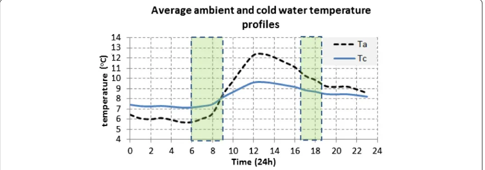
Case study 1
This case study compares results of two simulations. In the first simulation, we use actual values of ambient temperature Ta and cold water temperatures Tc, shown in Figure 14. Shaded areas indicate peak periods of hot water usage (06:00–09:00 and 16:30–18:30). The pro-file ofTais obtained from historical climate data for Tas-mania (October 2, Bureau of Meteorology and Australia 2012); Tcusually has a positive correlation withTa , van Harmelen and Delport (1999), but has a smaller range of variation. As can be seen in Figure 14, values ofTaand
Tc vary considerably over the 24-hour period (particu-larly, values of Ta), but their variations during peak pe-riods are rather small. Therefore, in the second simulation,TaandTcare set to constant value of 8°C.
Figure 15 shows two aggregate uncontrolled water heating load curves obtained using variable and constant values for ambient and cold water temperatures. We find insignificant difference between the two curves. The dif-ference in the total energy consumption is about 1%, and the mean absolute error (MAE) is about 1.3p.u. The results can be explained by the fact that a great majority of hot water usages occur during peak periods when var-iations of actual cold water temperature are rather small (within ± 1°C, in shaded areas of Figure 14). On the other hand, although Ta varies significantly during the day, its variation has negligible overall effect on the rate of hot water tank heat losses. An insulated hot water
tank idles for a long period (usually from 13 to 15 hours) between two consecutive recharges due to heat loss. During this period, the effect of Ta variation is smoothed, and the average value of Ta produces similar results as its variable values. Thus, variations of Ta and
Tc can be represented with their respective average values in further studies.
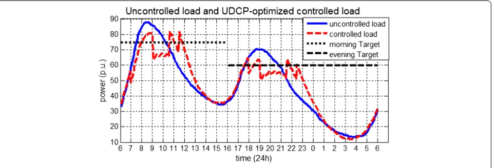
Case study 2
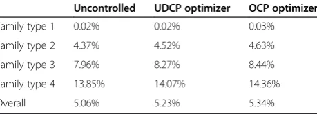
This case study compares the performance of the UDCP optimizer and the OCP optimizer. Both use the default switching program configuration to produce optimized switching programs that are applied to the same set of water heating loads. The peak reduction target is 15% in both cases. Figures 16 and 17 show the aggregate con-trolled load curves produced by the UDCP and OCP op-timizers, respectively. Table 4 shows the control periods and peak reductions achieved. The UDCP optimizer keeps user-specified control periods constant in its optimization process. Probabilities of cold showers for each family type are shown in Table 5–for the uncon-trolled scenario, and scenarios conuncon-trolled by the UDCP-optimized and OCP-UDCP-optimized switching programs.
Comparing the aggregate controlled load curves pro-duced by both optimizers, we find that the OCP optimizer performs much better in terms of peak load reduction.
The starting and finishing times of control periods in a switching program are vital for peak load reduction. A
Figure 18The OCP optimization of a water heating load profile with the dominant evening peak.
Table 6 Probabilities of cold showers for case study 3
Uncontrolled Controlled
Family type 1 0.03% 0.05%
Family type 2 4.11% 4.48%
Family type 3 7.50% 8.31%
Family type 4 14.32% 15.81%
Overall 4.82% 5.30%
Table 7 Switching program configurations in case study 4
Configuration 1 (default) Configuration 2
Control groups 6 3
Switching cycle 30 (min) 30 (min)
Control step 5 (min) 10 (min)
delayed control period produces an initial peak above the target line, as in the evening period of Figure 16. Starting a control period too early defers loads need-lessly and creates slightly higher peaks in subsequent switching cycles of the same control period, as in the morning control period of Figure 16. Control periods with sufficient length allow a gradual restoration of loads below the target line. Ending a control period prema-turely creates an unwanted high payback peak at the end of the control period, as seen at around 11:30 of Figure 16. Similar results were reported in Kondoh (2011), and Lee and Wilkins (1983). Due to shorter than required control periods used for the UDCP optimization, redu-cing the peaks at 10:30 and 21:30 will produce higher payback peaks at the end of the respective control periods.
While both controlled scenarios produce higher prob-abilities of cold shower than in the uncontrolled sce-nario, the OCP optimizer degrades the comfort level more than the UDCP optimizer due to its longer control periods (Table 5).
Case study 3
In this case study, we evaluate the tool’s ability to optimize switching programs for two different water heating load profiles. The first one has a dominant morning peak (this load profile was used in the case study 3) and the second – a dominant evening peak. The default switching program configuration (30 min switching cycle with 5-minute control steps and six con-trol groups) is used. The peak reduction target is 15%. Figure 18 shows the aggregate uncontrolled load curve of the second water heating load profile, and the aggre-gate controlled load curve after the OCP-optimized switching program is applied.
Optimized morning and evening control periods are from 07:30 to 15:00 and from 17:30 to 23:30, respectively.
A 9.1% peak reduction is achieved for the morning control period, and 13.4% for the evening. Table 6 shows probabilities of cold showers estimated for each family type under uncontrolled and controlled scenarios. As can be seen from Figure 18, the tool cannot further reduce the payback peak detected at 14:30 as the morning control period has reached the maximum limit of 7.5 hours.
Comparison of the results produced by the OCP optimizer in the case studies 2 and 3 (Tables 5 and 6) re-veals that customers experience similar comfort under different load profiles.
Case study 4
In this case study, we use the water heating load profile of case study 2 and compare two different switching programs represented in Table 7. Results produced by the OCP optimizer for case study 3 represent the imple-mentation of the default configuration. Results shown in Figure 19 represent the implementation of the second switching program (configuration 2), and Table 8 shows probabilities of cold showers estimated for each family type. The optimized control period is from 07:30 to 13:30 in the morning and from 17:30 to 00:00 in the evening. Peak reductions for morning and evening con-trol periods are 14.8% and 13.2%, respectively.
The default switching program configuration performs slightly better in peak reduction as it has smaller control
Figure 19The OCP optimization with the switching program configuration 2.
Table 8 Probabilities of cold showers for case study 4
Uncontrolled Controlled
Family type 1 0.02% 0.08%
Family type 2 4.37% 4.80%
Family type 3 7.96% 8.67%
Family type 4 13.85% 14.55%
steps and higher number of control groups. Switching program configuration 2 degrades the customer comfort level further as water heating systems are switched off for longer periods of time.
Conclusions
With a strong drive for energy conservation, demand re-sponse is becoming vital for the implementation of the smart grid concept. This paper outlines some experience obtained at University of Tasmania, Australia in develop-ing a DR visualization tool.
The visualization tool is designed to recommend optimum DR switching programs for domestic water heat-ing systems. The tool assesses the performance of a DR switching program by estimating potential peak load re-ductions and customer comfort characterized by the prob-ability of cold showers. The starting time and the length of control periods are crucial in peak reduction. However, the length of control periods must be limited to minimize negative impact on customer comfort. The developed tool aims to assist distribution system operators in designing their DR programs. The results are presented in a graph-ical form. An operator uses this tool to determine the available domestic water heating load in a controlled area, and predict the potential reduction in peak load. The tool described in this paper has been implemented in the Tas-manian power system since June 2013.
The developed tool has a modular structure, which en-ables it to be extended to cover air conditioners, pool pumps and electric vehicle charging load.
Competing interests
The authors declare that they have no competing interests.
Authors’contribution
Both authors share equally the work. MN led the research and drafted the manuscript. KW developed the tool and carried out the case studies. Both authors read and approved the final manuscript.
Acknowledgements
This work was supported in part by TasNetworks, Tasmania Australia. The authors gratefully acknowledge contributions of Peter Milbourne, James O’Flaherty, Daniel Capece, Cherry Wynn and Dr. Thanh Nguyen of TasNetworks, Australia for productive discussions of the results presented in this paper.
Received: 25 November 2014 Accepted: 28 January 2015
References
Australian Bureau of Statistics. (2012). Available: www.ausstats.abs.gov.au. Bureau of Meteorology, Australia. (2012). Available: www.bom.gov.au. Elphick, S, Ciufo, P, & Perera, S. (2009). Supply current characteristics of modern
domestic loads. InProceedings of the Australasian Universities Power
Engineering Conference(pp. 1–6).
Gomes, A, Martins, AG, & Figueiredo, R. (1999). Simulation-based assessment of electric load management programs.International Journal of Energy Research, 23, 169–181.
Gomes, A, Antunes, CH, & Martins, AG. (2004). A multiple objective evolutionary approach for the design and selection of load control strategies.IEEE
Transactions on Power Systems, 19, 1173–1180.
Heussen, K, You, S, Biegel, B, Hansen, L, & Andersen, K. (2012). Indirect control for demand side management-A conceptual introduction. InProceedings of the
3rd IEEE PES ISGT Europe(pp. 1–8).
Kondoh, J. (2011). Direct load control for wind power integration. InProceedings
of the IEEE PES General Meeting(pp. 1–8).
Kondoh, J, Lu, N, & Hammerstrom, DJ. (2011). An evaluation of the water heater load potential for providing regulation service. InProceedings of the IEEE PES
General Meeting(pp. 1–8).
Lee, S, & Wilkins, C. (1983). A practical approach to appliance load control analysis: a water heater case study. InIEEE trans. power apparatus and systems (pp. 1007–1013).
McKelvie, P., Hoddinott, Boland, G. and Kahl, G. (1992).“Load Management Tools for Optimal Control of Hot Water Loads,”Proceedings of the Electric Energy
Conference, 1992, pp. 153–159.
Negnevitsky, M, & Wong, K. (2015). Demand-side Management Evaluation Tool”.
IEEE Transactions on Power Systems, 30(1), 212–222.
Nehrir, MH, Jia, R, Pierre, DA, & Hammerstrom, DJ. (2007). Power management of aggregate electric water heater loads by voltage control. InProceedings of
the IEEE PES General Meeting(pp. 1–6).
Nguyen, DT, Negnevitsky, M, & de Groot, M. (2011). Pool-based demand response exchange—concept and modeling.IEEE Trans Power Systems, 26, 1677–1685. Ohnaka, T, Tochihara, Y, & Watanabe, Y. (1994). The effects of variation in body
temperature on the preferred water temperature and flow rate during showering.Ergonomics, 37, 541–546.
Strbac, G. (2008). Demand side management: benefits and challenges.Energy
Policy, 36, 4419–4426.
van Harmelen, G, & Delport, GJ. (1999). Multi-Level Expert-Modelling for the Evaluation of Hot Water Load Management opportunities in South Africa”.
IEEE Trans Power Systems, 14(4), 1306–1311.
van Tonder, JC, & Lane, IE. (1996). A load model to support demand management decisions on domestic storage water heater control strategy.
IEEE Transactions on Power Systems, 11, 1844–1849.
Wayne, M., and Gellings, C.W. (1984).“Demand Planning in the’80s”,EPRI Journal, Electric Power Research Institute.
Wong, K, & Negnevitsky, M. (2013). Development of an evaluation tool for demand side management of domestic hot water load. InProceedings of the
IEEE PES GM. Canada: Vancouver.
Submit your manuscript to a
journal and benefi t from:
7Convenient online submission
7Rigorous peer review
7Immediate publication on acceptance
7Open access: articles freely available online
7High visibility within the fi eld
7Retaining the copyright to your article