Refining deep convolutional features for improving fine-grained image recognition

(1)

R E S E A R C H

Open Access

Refining deep convolutional features for

improving fine-grained image recognition

Weixia Zhang

1

, Jia Yan

1

, Wenxuan Shi

2

, Tianpeng Feng

1

and Dexiang Deng

1*

Abstract

Fine-grained image recognition, a computer vision task filled with challenges due to its imperceptible inter-class variance and large intra-class variance, has been drawing increasing attention. While manual annotation can be utilized to effectively enhance performance in this task, it is extremely time-consuming and expensive. Recently, Convolutional Neural Networks (CNN) achieved state-of-the-art performance in image classification. We propose a fine-grained image recognition framework by exploiting CNN as the raw feature extractor along with several effective methods including a feature encoding method, a feature weighting method, and a strategy to better incorporate information from multi-scale images to further improve recognition ability. Besides, we investigate two dimension reduction methods and successfully merge them to our framework to compact the final image representation. Based on the discriminative and compact framework, we achieved the state-of-the-art performance in terms of classification accuracy on several fine-grained image recognition benchmarks based on weekly supervision.

Keywords:Fine-grained image recognition, Convolutional Neural Networks (CNN), Bag-of-visual-words, Feature weighting, Dimension reduction

1 Introduction

As a fashionable topic in computer vision, fine-grained image recognition has been attracting increasingly atten-tion from both academia and industry in the past few years. Taking identifying a bird as an example, it not only aims at pointing out whether the input image presenting a bird or something else (‘cat’,’dog,’’plant’,’car’etc.), but also the specifies of the bird (a‘albatross’or a‘cuckoo’, or even more exact, a‘black footed albatross’), which can only be discriminated by minute difference of physiological fea-ture. Besides, diverse postures, circumstances, viewpoints, positions, etc. may usually cause non-negligible interfer-ence for recognition, which further increase the difficulty. Therefore, compared with general object recognition, this task is rather challenging.

In view of the above annoying problems, part annota-tions, object bounding box or part annotations are often used to eliminate background noise and to highlight the discriminative part [1–6], such as the whole body, head, or torso of a bird. However, these manual labeling works are always extremely time-consuming, expensive, and

not completely accurate due to artificial error or diverse subjective cognition of the exact position information.

Without such expensive manual label information, powerful image representation will be the key factor for fine-grained visual recognition. Convolutional Neural Net-works (CNN)-based methods achieve state-of-the-art. FV-CNN [7] is initially proposed for texture recognition and has been shown to be also suitable for fine-grained visual recognition. One most appealing advantage of FV-CNN may be that it can incorporate multi-scale image informa-tion seamlessly. Bilinear CNN model (B-CNN) [8] extract features from non-linearity activations of convolutional layers from two CNN, achieving remarkable performance in fine-grained visual recognition without any bounding-box or part annotation. We propose our fine-grained image recognition framework based on FV-CNN and gear it with a novel strategy of utilizing multi-scale information. B-CNN, however, will be treated as an end-to-end model fine-tuning method in our framework. Besides, we investi-gate two dimension reduction methods: Tensor Sketch approximation [9] and Mutual Information dimension se-lection [10] to compact FV-CNN which is rather high-dimensional and cannot be generalized to large-scale task.

* Correspondence:[email protected]

1_{School of Electronic Information, Wuhan University, Wuhan, China} Full list of author information is available at the end of the article

(2)

Apart from powerful image representation, picking useful features in an unsupervised manner is another path to enhance performance. By an intuitive and he-uristic consideration, hand-crafted saliency detection technologies [11] might be a straightforward choice. However, most saliency detection are implemented on pixel level, which might detect salient region in human’s perspective, which is not necessary for a fine-grained

image recognition system. In a CNN’s pipeline,

numer-ous feature maps, which can be spatially mapped back to the original image, will be generated spontaneously. Be-cause the feature maps’values were obtained by an itera-tively optimization process which aim at achieving better recognition performance, they can be utilized to locate and extract discriminative descriptors of an image. In this line of thought, several works have already achieved good results [12–14]. In this paper, we propose a non-parametric feature weighting method based on refining convolutional descriptors to boost performance.

Overview of our proposed feature extraction frame-work is illustrated in Fig. 1.

The remainder of this paper is organized as follows: Section 2 describes related works. Our proposed strategy of utilizing multi-scale information is discussed in Sec-tion 3. In secSec-tion 4, we describe our feature processing in detail. Section 5 describes compact FV-CNN. Experi-ment results and analysis are given in Sections 6, and Section 7 concludes the paper.

2 Related works 2.1 FV-CNN

Bag-of-visual-words (BOW) model and its variants such as Fisher Vectors [15, 16] and VLAD [17, 18], and deep

learning led by Convolutional Neural Networks (CNNs) [19, 20] are two mainstreaming architecture for image classification. Pipelines of classical BOW and its variants are composed of four steps:

Firstly, extracting local descriptors, e.g., SIFT [21], HOG [22], LBP [23], etc.

Secondly, clustering the local descriptors by K-means or Gaussian mixture model (GMM) and forms a visual dictionary.

After that, repeating the first step for every test image and encoding them to a single feature vector based on histogram of occurrences of each terms in visual dictionary or storing the statistics of the difference between centers (K-means) or modes (GMM) and each descriptor.

Finally, feeding the encoded feature vectors to a classifier such as linear SVM and getting the classification result.

FV-CNN framework extract descriptors from the last con-volutional layer of a CNN to replace hand-crafted features, and the rest steps are similar to classical BOW model.

Although FV-CNN can incorporate multi-scales infor-mation, which has been shown to be an effective strategy to boost recognition performance, of an image in a seamlessly manner, its parameters, i.e., parameters of its GMM cannot be tuned like traditional CNN, which limit its performance.

2.2 Bilinear CNN (B-CNN)

Similar to FV-CNN, Bilinear CNN (B-CNN) also em-ploys convolutional features from CNN. In B-CNN, the

(3)

feature outputs are combined at each location of feature maps from rectified convolutional layer using the matrix outer product. Unlike FV-CNN, B-CNN can be trained by end-to-end learning, therefore, it also provides an al-ternative training method to traditional fully connected training (FC-CNN). Lin et al. employ B-CNN [8] to achieve remarkable performance in several fine-grained visual recognition benchmark datasets.

Despite that B-CNN is powerful, its final feature repre-sentation requires tremendous storage due to the ex-tremely high dimension (e.g., 262,144 dimensional per image on VGG-16). Gao et al. [24] proposed two compact B-CNN methods with the same discriminative power as the full bilinear representation with much less dimensions.

2.3 Feature weighting

Unsupervised discriminative region detection is crucial for fine-grained image recognition without object bounding-box and part annotations. Recently, Wei et al. proposed an architecture termed ‘Selective Convolutional

Descrip-tor Aggregation (SCDA)’ [13] to select useful

convolu-tional descriptor by feature maps from multiple layers in a CNN, which achieved good performance in both fine-grained retrieval and fine-fine-grained recognition. Zhang et al. [14] proposed a spatially weighted Fisher Vector (SWFV) for improving the performance of FV-CNN in fine-grained visual recognition task by spatially weighting Fisher Vectors.

3 Multi-scale feature

Inheriting from classical bag-of-visual-words model, FV-CNN pools multi-scale information from input image pyr-amids, i.e., different rescaled versions of a same original image, as shown in the flowing from part (a) to part (c) in Fig. 1. Although this classical technique is effective for im-proving recognition capability, it meets some limitations. In order to extract features from aP-level image pyramids, i.e., image pyramids consist of images withPdifferent res-olutions re-scaling from one original image, each of them should be fed into the CNN model and be processed by some preliminary operation such as convolution and pool-ing layer by layer, as shown in part (b) in Fig. 1, which brings large computation burden asPincreases especially in a very deep model such as VGG-16 [25]. Besides, the

way of generating multi-scale image features is simply based on resizing the input image by interpolation-based

methods such as bilinear interpolation or bicubic

interpolation; this is somewhat monotonous in terms of diversity of feature.

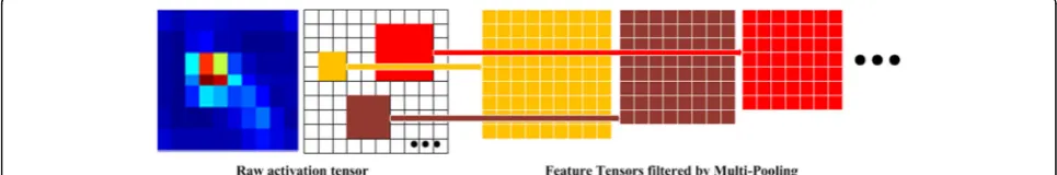
Facing these limitations, we propose to generate multi-scale information by pooling feature tensors of the last

convolutional layer with relu activation in a CNN using

different pooling window sizes, which is shown in the flowing of part (c) to part (d) in Fig. 1 and more detailed in Fig. 2. Compared with traditional image resizing method, which inputs a resized image to the CNN, and let it get through all layers in it, this one only get through one layer, i.e., a pooling layer, which needs much less computation, furthermore, the pooling oper-ation is substantially different from interpoloper-ation-based image resizing and thus it can enrich the multi-scale in-formation by jointly utilized with the former.

This proposed method can be explained in receptive fields. When a CNN is applied on an image, assume the size of the activation feature maps of last convolutional

layer is H×W×D, where H and W are the height and

width of the activation feature maps, respectively, and

the Ddenotes number of feature maps, i.e., the number

of channels. This activation structure can not only be seen asDfeature maps, but alsoH×Wspatially distributedD -dimensional descriptors. Each descriptor corresponds to a receptive field in the original image. Receptive fields with different sizes covers different content in original image, hence, this operation is in accordance with traditional multi-scale strategy by using image pyramids, both of which will generate more comprehensive information compared with single-scale image or single activation fea-ture map. The multi-pooling and image pyramids can also be jointly utilized in a straightforward way, i.e., applying multi-pooling to the raw activation feature maps of each image from the input image pyramid. For choice of pool-ing method, we use max-poolpool-ing here.

4 Feature processing 4.1 Feature encoding

Fisher Vectors [15, 16] and VLAD [17, 18] are two com-monly used features encoding in bag-of-visual-words framework. Given a trained Gaussian mixture model

(4)

(GMM) with parameter Θ = (μk, Σk, πk∈ ℝD ; k = 1, …,K) and K-means dictionary with centersc1,…,ck∈ℝD,

let I = (x1,…,xN) be a set of D-dimensional feature

de-scriptors extracted from an image, Fisher Vectors pools these descriptors byΦ(I) = [u1,…,uK,v1,…,vK], where:

ujk ¼ 1 Npffiffiffiffiffiπk

X

i¼1

N qik

xji−μjk

σjk ;

vjk¼

1 Npffiffiffiffiffiffiffiffi2πk

X

i¼1

N qik

xji−μjk

σjk

2

−1

" #

;

qik¼

exp −1 2 xi−μk

T_Σk−1

xi−μk

X

t¼1

K

exp −1 2ðxi−μtÞ

T_Σk−1

xi−μt

ð Þ

:

ð1Þ

omσjk is just the diagonal element of diagonal matrix Σk, and indexjspan all dimensions.ujkandvjkare accu-mulated sum of the first and second order statistics of descriptors xji respectively. Different from Fisher Vec-tors, VLAD only accumulate the first order statistics with K-means dictionary:

vjk¼

X

i¼1 N

qik xji−cjk

ð2Þ

Whereqikhere is usually obtained by nearest neighbor assignment methods such as approximate nearest neigh-bors (ANN).

Observing (1) and (2), it is clear that Fisher Vectors and VLAD are formulated differently and resort to dif-ferent visual dictionary, i.e., GMM and K-means, re-spectively. Instead of researching which encoding method is better, we propose to simply concatenate them to form a new vector which we term as VLAD-FV and can be formulated as:

φð Þ ¼I ½v1;…;vK;u1;…;uK; v1;…;vK ð3Þ

Taking their difference into account, they are expected to be complementary and thus their combination is ex-pected to have a better representation ability. We will empirically prove its effectiveness in Section 6.4.

4.2 Feature weighting

Original FV-CNN treat each convolutional descriptor equally and pool them by Fisher Vectors or by VLAD directly. However, in fine-grained image recognition task, the main objects are often confused or even oc-cluded by background and thus descriptors extracted from these useless or even harmful region are unfavor-able for recognition. We propose to alleviate this prob-lem by spatially weighting convolutional descriptors with

a clear purpose that highlight useful features and sup-press useless or harmful ones.

As discussed in Section 3, numerous feature maps are generated spontaneously in each layer in a CNN’s pipe-line. After a CNN model has been trained, the activation

of the last convolutional layer is a H×W×D tensor

which can be seen as H×W D-dimensional descriptors

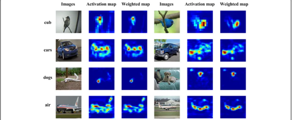
when they are used for feature encoding. On the other hand, if we treat it as D feature maps with sizeH×W, it can be observed that each channel responses to different parts semantically of the input image, as shown in Fig. 3. We pick some feature maps in the last convolutional layer after non-linearity activation and visualize them by simply normalizing their values. Obviously, some feature maps response highly to whole objects, e.g., 15th chan-nel of bird 1, 289th chanchan-nel of car 2, and some only re-spond to parts of correre-sponding objects, e.g., 136th channel of bird 2, 253th channel of dog 2, 109th channel of air 1 while some of them response to noisy back-ground, e.g., 413th channel of bird 2, 192th channel of air 1, 383th channel of air 2.

Considering discriminative regions usually have higher activation, and more feature maps will respond to them,

we propose to accumulate all feature maps along D

channels, then we obtain an activation map with a size

of H×W, then this activation map will be applied to

each feature map to complete the spatial weighting. Tak-ing VGG-16 as an example, firstly, we extract activation tensorA∈ℝH×W×Dof the last convolutional layer with relu activation, following by a max-pooling of stride 2,

we get an intermediate map matrix Win which usually

has size around H₂W₂. After that, it will be divided by the max value such that all values in it lie in the range [0, 1]. Then we do a square-rooting operation on the

map and obtain the Win (after dividing by max value),

and finally it is resized to H×W by nearest-neighbor

interpolation, and we get the final weighting map

W∈RH×W. The whole process is illustrated in (4):

Winð Þ ¼i; j

XD

t¼1

A ið; j; tÞ;

Win¼

ffiffiffiffiffiffiffiffiffiffiffiffiffiffiffiffiffiffiffiffiffiffiffiffiffiffiffiffiffiffiffiffiffiffiffiffiffiffi

Win=maxðWinð ÞS Þ

p

;

W ¼ ℕ ℕ ℝðWinÞ:

ð4Þ

whereSdenotes set of spatial locations of intermediate

map and ℕℕℝ denotes nearest neighbor

interpolation-based resizing.

(5)

all of them together with that weighted tensor from the original activation tensor by VLAD-FV.

5 Compact FV-CNN

We propose to concatenate Fisher Vectors and VLAD to form VLAD-FV, which inevitably increases dimension of image representation. Thus, effective dimension reduc-tion deserves to be researched. In view of this problem, we investigate two dimension reduction technologies.

5.1 MI dimension selection

A conclusion that strong linear correlation between two dimensions almost does not exist in Fisher Vec-tors or VLAD is obtained in [10]. Therefore, instead of compressing whole feature dimensions altogether, reducing dimension of Fisher Vectors and VLAD by

selecting useful dimensions deserves to be

investigated.

We denote image labels as y, the Fisher Vectors or

VLAD values in the ith dimension as x:i, and the

(6)

mutual information as I(x:i,y). The MI value repre-sents importance score for each dimension and is computed as:

I xð :i;yÞ ¼H xð Þ:i −H xð :i;yÞ; ð5Þ

Where H(x) is the entropy of a random variable. After the MI values for all dimensions are calculated, dimen-sions are re-ranked according to their MI values, and if

we want to reduce a D-dimensional feature tod

-dimen-sional, simply select the topd dimensions in sorted list. For more details of this off-the-shelf technology, one may refer to [10].

5.2 Tensor Sketch approximation

VLAD and Fisher Vectors are usually reshaped to single vectors for classification. For convenience of low-dimensional analysis, it is desirable to keep the original distribution of each entry as shown in Fig. 4. Inspired by B-CNN, FV-CNN can be transformed to another repre-sentation by matrix multiplication of a FV-CNN and its transposition:

Φfvð Þ ¼I ½u1; :::::::;uk;σ1; ::::::;σk;

Φvð Þ ¼I ½ν1; ::::::;νk;

Φvfvð Þ ¼I ½Φvð ÞI ;Φfvð ÞI ;

Φvfvtransformedð Þ ¼I Φvfvð Þ I Φvfvð ÞI T_;

ð6Þ

whereΦfv(I),Φv(I),Φv_fv(I) andΦv_fv_transformed(I) denotes Fisher Vectors, VLAD, VLAD-FV and transformed VLAD-FV, respectively.

The transformed FV-CNN can be viewed as linear

ker-nel machines. Let X and Y denote two sets of Fisher

Vectors or VLAD, compare them in image classification using linear classifier such as SVM is operated as follows:

Φð ÞX

ð Þ;ðΦð ÞY Þ

h i ¼ X

i∈S1 xixiT

*

;X

j∈S2 yjyjT

+

¼X

i∈S1

X

j∈S2

〈

xi;yj

E2

;

whereS1andS2denote locations of two sets of FV-CNN. It is clear that comparison of entries of FV-CNN of two

images is actually a second-order polynomial kernel, thus, methods for low-dimensional approximation of second-order polynomial kernel can be applied on it.Tensor Sketch

is an algorithm, and details of this can be found in [9].

6 Experiments

6.1 Dataset and measurement

In this section, we will use four fine-grained benchmarks to perform experimental evaluation:

Caltech-UCSD 2011 bird dataset (cub): it contains 11,788 images of 200 bird species.

FGVC-aircraft dataset [26] (air): it consists of 10,000 images of 100 aircraft categories.

FGVC-car dataset [27] (cars): it is composed of 16,185 images of cars from 196 classes.

Stanford dogs dataset [28] (dogs): 20,580 images with 120 dog species are included in it.

For all datasets, we follow the fixed training and test-ing split provided by themselves. We do not resort to any object bounding-box and part annotation on both training and testing time, only image labels are used.

Measurement for all experiments is the fraction of cor-rectly predicted images.

6.2 Networks

For fair comparison with another method, we use VGG-16 [25] to perform experiments on cub, air, and cars while AlexNet [29] for dogs. Both VGG-16 and AlexNet are fine-tuned by B-CNN based on pre-trained models on ImageNet. All of them converge (validation error rate stop decreasing) in less than 60 epoches, and we do not use any data augmentation in fine-tuning.

6.3 Implementation details

Images of cub have moderate size, and thus, we directly use the original size of them, while the size of the images from the other three datasets are rather variable and hence we normalize all their images to 448 × 448 × 3 firstly. We double the training data by horizontal flip-ping, and we average the predictions of a test image and its flipped copy, and we output the class with highest

(7)

score. Once feature extraction for all images is done, one-versus-all linear SVM classifiers will be trained with

constant learning hyperparameter C= 1 to perform

rec-ognition. The trained classifiers are recalibrated by chan-ging the SVM bias and rescaling the SVM weight vector such that median scores of the negative and positive

training examples are at −1 and +1, respectively.

Num-ber of clusters for GMM and K-means is fixed to 64. We implemented all experiments using MatConvNet [30] and VLfeat [31].

6.4 Results and comparisons

6.4.1 Feature encoding

First of all, we evaluate the effectiveness of VLAD-FV by comparing the classification accuracies of all datasets using Fisher Vectors, VLAD, and VLAD-FV.

As results shown in Table 1, VLAD-FV consistently outperforms both Fisher Vectors and VLAD alone, hence, in the rest of all experiments, we will use VLAD-FV as the feature encoding method. Results using VLAD-FV in this part will be used as the baseline in the next experiments.

6.4.2 Multi-scale feature

We evaluate the effectiveness of multi-pooling by three comparative experiments: using classical multi-scale strat-egy by image pyramid, using multi-pooling on single scale image and both of them, i.e., the multi-pooling of image pyramids. Experimental results are shown in Table 2 from which we observe using multi-pooling on single image and on image pyramids that can boost recognition ability. For image pyramids, we use six scales with re-scaling fac-tor [0.5, 0.75, 1, 1.25, 1.5, 1.75]. For cub, the facfac-tor 1 repre-sents original image size, and for the other three datasets,

it represents images rescaled to 4484483

before-hand. We use six levels of multi-pooling because we find

that with this parameter, we achieve best performance in all datasets.

6.4.3 Descriptors weighting

Two experiments are presented in this part. Firstly, we evaluate descriptor weighting alone and then we evaluate using descriptors weighting along with multi-pooling strategy. In Table 3, we see the effectiveness of descrip-tors weighting, and its concordance with multi-pooling.

6.4.4 Dimension reduction

Experiments in this part is composed of four groups: dimension reduction by MI, dimension reduction by Tensor Sketch, dimension reduction by jointly using MI and Tensor Sketch, and widely used principal component analysis (PCA) where we project original descriptors from 512-dimensional to 24-dimensional such that the dimension of the final feature vector will be 24 × 64 + 24 × 2 × 64 = 4608 and being compar-able to other methods. All operations here are based on the best practices used above, i.e., multi-pooling of image pyramid with spatially weighted descriptors encoded by VLAD-FV. For MI selection, we present two results using two different numbers of selected dimensions because we find that when we carefully select useful dimensions (69,992 for VGG-16 and 40,000 for AlexNet), the accuracy may even improve while if we simply select a few dimension (4096 here) the performance drops violently.

From Table 4, we can see that jointly using tensor

sketch and MI consistently outperforms solely using either of them. It also has a better performance than widely used dimension reduction method PCA.

6.4.5 Comparison with other methods

Comparison with other methods in this part is twofold; in terms of accuracy and jointly considering accuracy and dimension of feature vector. For later, we define an

index-termed discriminative per dimension and

abbrevi-ated to DPD, which can be explained as discriminative power of a single dimension for better evaluating the ef-fectiveness of dimension reduction method. This is cal-culated as follows:

Table 1Comparison of performance of Fisher Vectors, VLAD, and VLAD-FV

Encoding methods Cub (%) Air (%) Cars (%) Dogs (%)

Fisher Vectors 79.0 82.3 83.7 64.1

VLAD 80.8 83.0 87.1 65.8

VLAD-FV 82.0 84.1 88.5 67.5

Table 2Evaluation of multi-pooling

Multi-scale strategy Cub (%) Air (%) Cars (%) Dogs (%)

Baseline 82.0 84.1 88.5 67.5

Image pyramid 84.9 85.8 90.3 69.7

Multi-pooling of single image 84.2 85.2 89.9 68.6

Multi-pooling of image pyramid 85.6 86.5 91.3 71.4

Table 3Evaluation of descriptors weighting

Methods Cub

(%) Air (%)

Cars (%)

Dogs (%)

Baseline 82.0 84.1 88.5 67.5

Descriptors weighting 83.6 85.4 90.3 68.7

Descriptors weighting+multi-pooling

(8)

DPD¼CACC

D ; ð8Þ

where ACC and Ddenote classification accuracy and di-mension of feature vector of corresponding method, respect-ively.Cis a constant which we set to 8000 in this paper.

6.5 Discussion

Based on the above experimental results, several conclu-sions can be obtained:

VLAD-FV can be used instead as an off-the-shelf encoding method to improve classification accuracy when Fisher Vector or VLAD is going to be used. Difference of formulation and used visual dictionar-ies make Fisher Vector and VLAD being comple-mentary and thus can be concatenated to form a more powerful representation.

The proposed multi-pooling of convolutional activa-tion tensor can either be used alone which is very efficient or with traditional image pyramid multi-scale strategy which has better performance in terms of classification accuracy.

Descriptor weighting can boost performance

because it highlights discriminative feature and suppresses useless background information. For better illustrating, the reason why this simple weighting is effective, we sample a few images from all evaluated datasets and visualize their activation map referenced in (4) and activation map after weighting which is shown in Fig.5. We can see that compared with original activation maps, the weighted maps respond more on discriminative parts, and activation on background are attenuated.

From Table5, we conclude that while tensor sketch sorts to conserve discriminative power using as few dimension as possible, MI emphasizes on selecting the most useful information in a given dimension. Thus, jointly using them is preferred when both discriminative power and compact representation are pursued. Although both MI dimension selection andtensor sketch approximationare existing methods, there are two points that deserve to be noted: firstly, to the best of our knowledge, we are the first to apply tensor sketch on Fisher Vectors and VLAD (for VLAD-FV, tensor sketch is applied on VLAD part and Fisher Vectors part separately,

Table 4Evaluation of dimension reduction. For dogs, we use AlexNet and thus the dimension of full vector of this is 49,152

Strategy Cub (%) Air (%) Cars (%) Dogs (%) Dimension

Full vector 86.3 87.5 92.1 72.3 98,304/49,152

Tensor Sketch 84.9 83.4 88.9 69.6 12,288

MI Selection 1 75.3 73.6 81.8 63.9 4,906

MI Selection 2 86.4 87.7 92.4 72.6 69,992/40,000

Tensor Sketch + MI 84.5 82.5 87.5 68.4 4,906

PCA 82.3 81.0 85.2 65.6 4,608

(9)

and their approximated vectors will be

concatenated); secondly, we are the first to jointly apply these two technologies to compact final image representation.

Some state-of-the-art methods are still very competi-tive, but our framework has its own advantages. Com-pared with [3,4,12], our framework do not rely on any

bounding-box or part annotations and achieve similar or even better results; compared with [8,24,32], be-cause we use FV-CNN as our baseline, our framework has better ability to incorporate multi-scale information and achieve better performance in the end; compared with [14,33], we do not need to train an extra part de-tector, which are always non-trivial.

Table 5Comparison of performance of our methods with some recent state-of-the-art methods in cub. BBox, parts denote bounding-box and parts annotation respectively

Methods Train phase Test phase Dim. Model Acc. DPD

Dataset: cub

Part-stacked CNN [1] BBox+Parts BBox 4,096 Part-Stacked CNN 76.2% 1.484

Deep LAC [2] BBox+Parts BBox 12,288 Alex-Net 80.3% 0.521

PN-CNN [3] BBox+Parts n/a 13,512 Alex-Net 85.4% 0.506

PG-alignment [4] BBox n/a 126,976 VGG-19 82.8% 0.052

Symbolic [5] BBox BBox 20,992 Shallow feature: SIFT 59.4% 0.226

Cross layer pooling[6] BBox BBox Alex-Net 73.5% 1.436

Mask-CNN [12] Parts n/a 8192 VGG-16+FCN 85.4% 0.834

Spatial transformer CNN [32] n/a n/a ST-CNN 84.1% 1.643

Bilinear CNN [8] n/a n/a 262,144 VGG-16+VGG-M 84.1% 0.026

Compact bilinear CNN [24] n/a n/a 8,192 VGG-16 84.0% 0.820

PD+SWFV [14] n/a n/a 69,632 VGG-16 84.5% 0.097

SCDA [13] n/a n/a VGG-16 80.5% 1.572

Ours n/a n/a 69,992 VGG-16 86.4% 0.099

Ours (compact vector) n/a n/a VGG-16 84.5% 1.650

Dataset: air

Re-Fisher Vector [34] n/a n/a 655,360 Shallow feature: SIFT 81.5% 0.001

Ours (Full Vector + MI 2) n/a n/a 69,992 VGG-16 87.7% 0.100

Dataset: cars

PG-Alignment [4] BBox n/a 126,976 VGG-19 92.6% 0.058

Ours n/a n/a 69,992 VGG-16 92.4% 0.106

Dataset: dogs

Selective pooling [35] BBox BBox 163,840 Shallow feature: SIFT 52.0% 0.025

NAC[33] n/a n/a Alex-Net 68.6% 1.340

PD+SWFV [14] n/a n/a 36,864 Alex-Net 71.9% 0.156

Ours n/a n/a 40,000 Alex-Net 72.6% 0.145

Ours (compact vector) n/a n/a Alex-Net 68.4% 1.335

(10)

7 Conclusions

In conclusion, the main contribution of this paper lie in four aspects: firstly, we propose a novel multi-scale strategy which can be utilized efficiently alone or together with classical image pyramids strategy which has better performance in terms of classification accuracy; secondly, we propose VLAD-FV to encode deep convolutional descriptors by concatenat-ing Fisher Vectors and VLAD, resultconcatenat-ing in better perform-ance than only using either of them; thirdly, VLAD-FV is rather high-dimensional and thus we apply two dimension re-duction methods to compact final image representation; last, but not the least, we propose a feature weighting method in descriptor level, which further enhances the performance.

Acknowledgements

None.

Funding

None.

Authors’contributions

WZ constructed the main ideas of the research, carried out most

experiments, and drafted the original manuscript. JY and WS took part in the examination of the study and participated in revising the manuscript. TF and DD offered useful suggestions in conducting experiments and drafting the manuscript. All authors read and approved the final manuscript.

Competing interests

The authors declare that they have no competing interests.

Publisher’s Note

Springer Nature remains neutral with regard to jurisdictional claims in published maps and institutional affiliations.

Author details

1_{School of Electronic Information, Wuhan University, Wuhan, China.}2_School of Remote Sensing and Information Engineering, Wuhan University, Wuhan, China.

Received: 14 September 2016 Accepted: 14 March 2017

References

1. S Huang, Z Xu, D Tao, Y Zhang, Part-stacked CNN for fine-grained visual categorization, inProceedings of the IEEE Conference on Computer Vision and Pattern Recognition (CVPR), 2016

2. D Lin, X Shen, C Lu, J Jia, Deep LAC: Deep localization, alignment and classification for fine-grained recognition, inProceedings of the IEEE Conference on Computer Vision and Pattern Recognition(CVPR), 2015, pp. 1666_–1674

3. S Branson, G Van Horn, S Belongie, P Perona, Bird specifies categorization using pose normalized deep convolutional nets, inProceedings of The British Machine Vision Conference (BMVC), 2014

4. J Krause, H Jin, J Yang, L Fei Fei, Fine-grained recognition without part annotations, inProceedings of the IEEE Conference on Computer Vision and Pattern Recognition(CVPR), 2015, pp. 5546–5555

5. Y Chai, V Lempitsky, A Zisserman, Symbiotic segmentation and part localization for fine-grained categorization. IEEE Int Conf Comp Vision 163(3), 321–328 (2013)

6. L Liu, C Shen, A van den Henge, The treasure beneath convolutional layers: Cross-convolutional-layer pooling for image classification, inProceedings of the IEEE Conference on Computer Vision and Pattern Recognition(CVPR), 2014, pp. 4749_–4757 7. M Cimpo, S Maji, A Vedaldi, Deep filter banks for texture recognition,

description and segmentation. Int J Comput Vis188(1), 65–94 (2016) 8. T.Y. Lin, A. RoyChowdhury, S. Maji. Bilinear CNN models for fine-grained

visual recognition. InIEEE International Conference on Computer Vision (ICCV), 1449–1457, 2015

9. N Pham, R Pagh, Fast and scalable polynomial kernels via explicit feature maps, inProceedings of the 19th ACM SIGKDD international conference on Knowledge discovery and data mining, 2013, pp. 239–247

10. Y Zhang, JX Wu, JF Cai, Compact representation of high-dimensional feature vectors for large-scale image recognition and retrieval. IEEE Trans Image Process25(5), 2407_–2419 (2016)

11. A Borji, MM Cheng, H Jiang, J Li, Salient object detection: a benchmark. IEEE Trans Image Process24(12), 5706–5722 (2015)

12. X. S. Wei, C-W. Xie, J. X. Wu. Mask-CNN: Localizing parts and selecting descriptors for fine-grained image recognition. arxiv.org, 1605.06878, 2016. 13. X.S. Wei, J.H Luo and J.X. Wu. Selective convolutional descriptor aggregation

for fine-grained image retrieval. arXiv:1604.04994,2016.

14. X Zhang, H Xiong, W Zhou, W Lin, Q Tian, Picking deep filter responses for fine-grained image recognition, inProceedings of the IEEE Conference on Computer Vision and Pattern Recognition(CVPR), 2016

15. F. Perronnin, J. Sánchez, and T. Mensink. Improving the fisher kernel for large-scale image classification. InEuropeon Conference on Computer Vision(ECCV), 143_–156. Springer, 2010.

16. F Perronnin, C Dance, Fisher kernels on visual vocabularies for image categorization, inProceedings of the IEEE Conference on Computer Vision and Pattern Recognition(CVPR), 2007, pp. 1–8

17. H Jégou, M Douze, C Schmid, P Pérez,IEEE Conference on Computer Vision and Pattern Recognition(CVPR), 2010, pp. 3304–3311

18. R Arandjelovi´c, A Zisserman, All about VLAD, inProceedings of the IEEE Conference on Computer Vision and Pattern Recognition(CVPR), 2013 19. A. Razavian, H. Azizpour, J. Sullivan, and S. Carlsson. CNN Features off-the-shelf:

an astounding baseline for recognition. CoRR, vol. abs/1403.6382, 2014. 20. K Chatfield, K Simonyan, A Vedaldi, A Zisserman, Return of the devil in the

details: delving deep into convolutional nets, inProceedings of The British Machine Vision Conference (BMVC), 2014

21. D. G. Lowe. Object recognition from local scale-invariant features. InThe proceedings of the seventh IEEE international conference on Computer Vision (ICCV). 2:1150–1157,1999

22. N Dalal, B Triggs, Histograms of oriented gradients for human detection. Proc IEEE Conf Comput Vis Pattern Recognit1, 886–893 (2005) 23. T Ojala, M Pietikinen, D Harwood, A comparative study of texture

measures with classification based on feature distributions. Pattern Recogn29(1), 51_–59 (1998)

24. Y Gao, O Beijbom, N Zhang, T Darrell, Compact bilinear pooling, in Proceedings of the IEEE Conference on Computer Vision and Pattern Recognition (CVPR), 2016

25. K. Simonyan and A. Zisserman. Very deep convolutional networks for large-scale image recognition.CoRRabs/1409.1556,2014.

26. S. Maji, E. Rahtu, J. Kannala, M. Blaschoko and A. Vedaldi. Fine-grained visual classification of aircraft.arXiv:1306.5151,2013

27. J Krause, M Stark, J Deng, L Fei-Fei, 3d object representation for fine-grained categorization, in3D Representations and Recognition Workshop, The proceedings of the seventh IEEE international conference on Computer Vision (ICCV), 2013

28. A Khosla, N Jayadevaprakash, B Yao, L Fei-Fei, Novel dataset for fine-grained image categorization, inProceedings of the IEEE Conference on Computer Vision and Pattern Recognition (CVPR), 2011

29. A. Krizhevsky, I. Sutskever and G. Hinton. ImageNet classification with deep convolutional neural networks.Advances in Neural Information Processing Systems, 25(2):1097-1105,2012

30. A. Vedaldi and K. Lenc. MatConvNet: Convolutional neural networks for MATLAB, 2014. Software available at http://www.vlfeat.org/matconvnet/. 31. A. Vedaldi and B. Fulkerson. VLFeat: An open and portable library of computer

vision algorithms, 2008. Software available at http://www.vlfeat.org/. 32. M. Jaderberg, K. Simonyan, A. Zisserman and K. Kavukcuoglu. Spatial

transformer networks. InConference and Workshop on Neural Information Processing Systems(NIPS).2008_–2016, 2015

33. M Simon, E Rodner, Neural activation constellations: unsupervised part model discovery with convolutional networks, inThe proceedings of the seventh IEEE international conference on Computer Vision (ICCV), 2015, pp. 1143–1151 34. P. H. Gosselin, N. Murray, H. Jégou and F. Perronnin. Revisiting the fisher

vector for fine-grained classification. Pattern Recognition Letters, Elsevier, 49, pp.92-98, 2014