Volume 2008, Article ID 274349,21pages doi:10.1155/2008/274349
Research Article
Feature Classification for Robust Shape-Based Collaborative
Tracking and Model Updating
M. Asadi, F. Monti, and C. S. Regazzoni
Department of Biophysical and Electronic Engineering, University of Genoa, Via All’Opera Pia 11a, 16145 Genoa, Italy
Correspondence should be addressed to M. Asadi,[email protected]
Received 14 November 2007; Revised 27 March 2008; Accepted 10 July 2008
Recommended by Fatih Porikli
A new collaborative tracking approach is introduced which takes advantage of classified features. The core of this tracker is a single tracker that is able to detect occlusions and classify features contributing in localizing the object. Features are classified in four classes: good, suspicious, malicious, and neutral. Good features are estimated to be parts of the object with a high degree of confidence. Suspicious ones have a lower, yet significantly high, degree of confidence to be a part of the object. Malicious features are estimated to be generated by clutter, while neutral features are characterized with not a sufficient level of uncertainty to be assigned to the tracked object. When there is no occlusion, the single tracker acts alone, and the feature classification module helps it to overcome distracters such as still objects or little clutter in the scene. When more than one desired moving objects bounding boxes are close enough, the collaborative tracker is activated and it exploits the advantages of the classified features to localize each object precisely as well as updating the objects shape models more precisely by assigning again the classified features to the objects. The experimental results show successful tracking compared with the collaborative tracker that does not use the classified features. Moreover, more precise updated object shape models will be shown.
Copyright © 2008 M. Asadi et al. This is an open access article distributed under the Creative Commons Attribution License, which permits unrestricted use, distribution, and reproduction in any medium, provided the original work is properly cited.
1. INTRODUCTION
Target tracking in complex scenes is an open problem in many emerging applications, such as visual surveillance, robotics, enhanced video conferencing, and sport video highlighting. It is one of the key issues in the video analysis chain. This is because the motion information of all objects in the scene can be fed into higher-level modules of the system that are in charge of behavior understanding. To this end, the tracking algorithm must be able to maintain the identities of the objects.
Maintaining the track of an object during an inter-action is a difficult task mainly due to the difficulty in segmenting object appearance features. This problem affects both locations and models of objects. The vast majority of tracking algorithms solve this problem by disabling the model updating procedure in case of an interaction. However, the drawback of these methods arises in case of a change in objects appearance during occlusion.
While in case of little clutter and few partial occlusions it is possible to classify features [1, 2], in case of heavy interaction between objects, sharing trackers information can help to avoid the coalescence problem [3].
In this work, a method is proposed to solve these prob-lems by integrating an algorithm for feature classification, which helps in clutter rejection, in an algorithm for the simultaneous and collaborative tracking of multiple objects. To this end, the Bayesian framework developed in [2] for shape and motion tracking is used as the core of the single object tracker. This framework was shown to be a suboptimal solution with respect to the single-target-tracking problem, where a posterior probabilities of the object position and the object shape model are maximized separately and suboptimally [2]. When an interaction occurs among some objects, a newly developed collaborative algorithm, capable of feature classification, is activated. The classified features are revised using a collaborative approach based on the rationale that each feature belongs to only one object [4].
The contribution of this paper is to introduce a collabo-rative tracking approach which is capable of feature classifi-cation. This contribution can be seen as three major points.
(2) Collaborative position estimation. The performance of the collaborative tracker is improved using the refined classes.
(3) Collaborative shape updating. While the methods available in literature are mainly interested in the col-laborative estimation, the proposed method imple-ments a collaborative appearance updating.
The rest of the paper is organized as follows. Section 2
discusses the related works. Section 3 describes the single-tracking algorithm and its Bayesian origin. InSection 4, the collaborative approach is described. Experimental results are presented inSection 5. Finally inSection 6some concluding remarks are provided.
2. RELATED WORK
Simultaneous tracking of visual objects is a challenging problem that has been approached in a number of different ways. A common approach to solve the problem is the Merge-Split approach: in an interaction, the overlapping objects are considered as a single entity. When they separate again, the trackers are reassigned to each object [5,6]. The main drawbacks of this approach are the loss of identities and the impossibility of updating the object model.
To avoid this problem, the objects should be tracked and segmented also during occlusion. In [7], multiple objects are tracked using multiple independent particle filters. In case of independent trackers, if two or more objects come into proximity, two common problems may occur: “labeling problem” (the identities of two objects are inverted) and “coalescence problem” (one object hijacks more than one tracker). Moreover, the observations of objects that come into proximity are usually confused and it is difficult to learn the object model correctly. In [8] humans are tracked using a priori target model and a fixed 3D model of the scene. This allows the assignment of the observations using depth ordering. Another common approach is to use a joint-state space representation that describes contemporarily the joint state of all objects in the scene [9–13]. Okuma et al. [11] use a single particle filter tracking framework along with a mixture density model as well as an offline learned Adaboost detector. Isard and MacCormick [12] model persons as cylinders to model the 3D interactions. Although the above-mentioned approaches can describe the occlusion among targets correctly, they have to model all states with exponential complexity without considering that some trackers may be independent. In the last few years, new approaches have been proposed to solve the problem of the exponential complexity [5, 13, 14]. Li et al. [13] solve the complexity problem using a cascade particle filter. While good results are reported also in low-frame rate video, their method needs an offline learned detector and hence it is not useful when there is no a priori information about the objects class. In [5], independent trackers are made collaborative and distributed using a particle filter framework. Moreover, an inertial potential model is used to predict the tracker motion. It solves the “coalescence problem,” but since global features are used
without any depth ordering, updating is not feasible during occlusion. In [14], a belief propagation framework is used to collaboratively track multiple interacting objects. Again, the target model is learned offline.
In [15], the authors use an appearance-based reasoning to track two faces (modeled as multiple view templates) during occlusion by estimating the occlusion relation (depth ordering). This framework seems limited to two objects and since it needs multiple view templates and the model is not updated during tracking, it is not useful when there is no a priori information about the targets. In [16], three Markov random fields (MRFs) are coupled to solve the tracking problem: a field for the joint state of multiple targets; a binary random process for the existence of each individual target; and a binary random process for the occlusion of each dual adjacent target. The inference in the MRF is solved by using particle filtering. This approach is also limited to a predefined class of objects.
3. SINGLE-OBJECT TRACKER AND
BAYESIAN FRAMEWORK
The role of the single tracker—introduced in [2]—is to estimate the current state of an object, given its previous state and current observations. To this end, a Bayesian framework is presented in [2]. The framework also is briefly introduced here.
Initialization
A desired object is specified with a bounding box. Then, all corners, say M, inside the bounding box are extracted and they are considered as the object features. They are shown asXc,t = {Xmc,t}1≤m≤M = {(xmt ,ymt )}1≤m≤M where the pair (xmt ,ymt ) is the absolute coordinates of corner m and the subscriptcdenotescorner. A reference point, for example, the center of the bounding box, is chosen as the object position. In addition, an initialpersistencyvaluePIis assigned to each corner. It is used to show the consistency of that corner during time.
Target model
The object shape model is composed of two elements:Xs,t = {Xms,t}1≤m≤M = {[DXmc,t,Pmt ]}1≤m≤M. The element DXmc,t =
Xmc,t−Xp,tis the relative coordinates of cornermwith respect to the object positionXp,t=(xreft ,yreft ). Therefore, the object status at timetis defined asXt= {Xs,t,Xp,t}.
Observations
Probabilistic Bayesian framework
In the probabilistic framework, the goal of the tracker is to estimate the posterior p(Xt | Zt,Xt−1 = X∗t−1). In this
paper, random variables are vectors and they are shown using bold fonts. When the value of a random variable is fixed, an asterisk is added as a superscript of the random variable. Moreover, for simplification, the fixed random variables are replaced just by their values: p(Xt | Zt,Xt−1 = X∗t−1) =
p(Xt | Zt,X∗t−1). Moreover, at timetit is supposed that the
probability of the variables at timet−1 has been fixed. The other assumption is that since Bayesian filtering propagates densities and in the current work no density or error propagation is used, the probabilities of the random variables at timet−1 are redefined as Kronecker delta functions, for example,p(Xt−1)=δ(Xt−1−X∗t−1). Using Bayesian filtering
approach and considering the independence between shape and motion one can write [2]
pXt|Zt,Xt∗−1
=pXp,t,Xs,t|Zt,X∗p,t−1,X∗s,t−1
=pXs,t|Zt,X∗p,t−1,X∗s,t−1,Xp,t
·pXp,t|Zt,X∗p,t−1,X∗s,t−1
. (1)
Maximizing separately each of the two terms at the right-hand side of (1) provides a suboptimal solution to the problem of estimating the posterior ofXt. The first term is the posterior probability of the shape object model (shape updating phase). The second term is the posterior probability of the object global position (object tracking).
3.1. The global position model
The posterior probability of the object global position can be factorized into a normalization factor, the position prediction model (a priori probability of the object position), and the observation model (likelihood of the object position) using the chain rule and considering the independence between shape and model [2]:
pXp,t|Zt,Xp∗,t−1,X∗s,t−1
=k·pXp,t|X∗p,t−1
·pZt|X∗p,t−1,X∗s,t−1,Xp,t
. (2)
3.1.1. The position prediction model (the global motion model)
The prediction model is selected with the rationale that an object cannot move faster than a given speed (in pixels). Moreover, defining different prediction models gives different weights to different global object positions in the plane. In this paper, a simple global motion prediction model of a uniform windowed type is used:
pXp,t|X∗p,t−1
= ⎧ ⎪ ⎪ ⎨ ⎪ ⎪ ⎩
1 Wx·Wy
ifXp,t−X∗p,t−1
≤W
2,
0 elsewhere,
(3)
whereWis a rectangular areaWx×Wyinitially centered on
X∗p,t−1. If more a priori knowledge about the object global
motion is available, it will be possible to assign different probabilities to different positions inside the window using different kernels.
3.1.2. The observation model
The position observation model is defined as follows:
pZt|X∗p,t−1,X∗s,t−1,Xp,t
= 1−e−Vt(Xp,t,Zt,X
∗
p,t−1,X∗s,t−1)
Zt 1−e
−Vt(Xp,t,Zt,X∗p,t−1,X∗s,t−1) ,
(4)
whereVt(Xp,t,Zt,X∗p,t−1,Xs∗,t−1) is the number of votes to a
potential object position. It is defined as follows:
Vt
Xp,t,Zt,X∗p,t−1,X∗s,t−1
= N
n=1 M
m=1
KR
dm,n
Xmc,t−1−X∗p,t−1,Znt −Xp,t
, (5)
where dm,n(·) is the Euclidean distance metric and it evaluates the distance between a model element mand an observation elementn. If this distance falls within the radius RR of a position kernel KR(·), mandn will contribute to increase the value of Vt(·) based on the definition of the kernel. It is possible to have different types of kernels, based on the a priori knowledge about the rigidity of desired objects. Each kernel has a different effect on the amount of the contribution [2]. Having a look at (5), it is seen that an observation element n may match with several model elements inside the kernel to contribute to a given position
Xp,t. The fact that a rigidity kernel is defined to allow possible distorted copies of the model elements contribute to a given position is called regularization. In this work, a uniform kernel is defined:
KR
dm,n
Xm
c,t−1−X∗p,t−1,Znt −Xp,t
= ⎧ ⎨ ⎩
1 ifdm,n
Xmc,t−1−X∗p,t−1,Znt −Xp,t
≤RR, 0 otherwise.
(6)
The proposed suboptimal algorithm fixes as a solution the valueXp,t=X∗p,tthat maximizes the product in (2).
3.1.3. The hypotheses set
To implement the object position estimation, (5) is imple-mented. Therefore, it provides an estimation for each point
A B
C F
D E
(a)
A B
C F
D E
(b) X∗p,t−1 Xp,t,1
Xp,t,2
(c)
(d) (e)
Figure1: (a) An object model with six model corners at timet−1. (b) The same object at timetalong with distortion of two corners “D” and “E” by one pixel in the direction ofy-axis. Blue and green arrows show voting to different positions. (c) The motion vector of the
reference point related to both candidates in (b). (d) The motion vector of the reference point to a voted position along with regularization. (e) Clustering nine motion hypotheses in the regularization process using a uniform kernel of radius√2.
to sufficiently high values of the estimated function (high number of votes) and they are spatially well separated. In this way, it can be shown that a set of possible alternative motion hypotheses of the object are considered corresponding to each selected point. As an example, one can have a look at
Figure 1.
Figure 1(a)shows an object with six corners at timet−1. The corners and the reference point are shown with red color and light blue, respectively. The arrows show the position of the corners with respect to the reference point.Figure 1(b)
shows the same object at time t, while two corners “D” and “E” are distorted by one pixel in the direction of y-axis. The dashed lines indicate the original figure without any change. For localizing the object, all six corners vote based on the model corners. In Figure 1(b), only six votes are shown without considering regularization. The four blue arrows show the votes of corners “A,” “B,” “C,” and “F” for a position indicated by the light blue color. This position can be a candidate for the new reference point and is shown by
Xp,t,1inFigure 1(c). Two corners “E” and “D” are voting to
another position marked with a green-colored circle. This position is called Xp,t,2 and it is located below the Xp,t,1
with a distance of one pixel.Figure 1(c)plotted the reference point at timet−1 and the two candidates at timetin the same Cartesian system. Black arrows inFigure 1(c)indicate the displacement of the old reference point considering each candidate at time t to be the new reference point. These three figures make the aforementioned reasoning clearer. From the figures, it is clear that each position in the voting space corresponds either to one motion vector (if there is no regularization) or to a set of motion vectors (if there is regularization (Figures1(d)and1(e))). Each motion vector, in turn, corresponds to a subset of observations that are moving with the same motion. In case of regularization,
these two motion vectors can be clustered together since they are very close. This is shown in Figures1(d)and1(e). In case of using a uniform kernel with a radius of√2 (6), all eight pixels around each position are clustered in the same cluster as the position. Such a clustering is depicted in Figures 1(d) and 1(e) where the red arrow shows the motion of the reference point at time t−1 to a candidate position.Figure 1(e)shows all nine motion vectors that can be clustered together. Figures1(d) and1(e)are equivalent. In the current work, a uniform kernel with a radius of √
8 is used (therefore, 25 motion hypotheses are clustered together).
To limit the computational complexity, a limited number of candidate points, sayh, are chosen (in this paperh=4). If the function produced by (5) is unimodal, only the peak is selected as the only hypothesis, and hence the new object position. If it is multimodal, four peaks are selected using the method described in [1,2]. Thehpoints corresponding to the motion hypotheses are calledmaximaand the hypotheses set is calledthe maxima set,HM= {X∗p,t,h|h=1· · ·4}.
In the current paper, the point inHM with the highest number of votes is chosen as the new object position (the winner). Then, other maxima in the hypotheses set are evaluated based on their distance from the winner. Any maximum that is close enough to the winner is considered as a member of the pool of winners WS and the maxima that are not in the pool of winners are considered as far maxima forming thefar maximasetFS=HM−WS.However, having a priori knowledge about the object motion makes it is possible to choose other strategies for ranking the four hypotheses. More details can be found in [1,2]. The next step is to classify features (hereinafter referred to as corners) based on the pool of winners and thefar maxima set.
3.1.4. Feature classification
Now, all observations must be classified, based on their votes to the maxima, to distinguish between observations that belong to the distracter (FS) and other observations. To do this, the corners are classified into four classes: good, suspicious, malicious, and neutral. The classes are defined in the following way.
Good corners
Good corners are those that have voted at least for one maximum in the “pool of winners” but they have not voted for any maximum in the “far maxima” set. In other words, good corners are subsets of observations that have motion hypotheses coherent with the winner maximum. This class is shown bySGas follows:
SG=
i=1···N(WS)
Si−
j=1···N(FS)
Sj, (7)
whereSiis the set of all corners that have voted for theith maximum andN(WS) andN(FS) are the number of maxima in the “pool of winners” and “far maxima set” respectively.
Suspicious corners
Suspicious corners are those that have voted at least for one maximum in the “pool of winners” and they have also voted for at least one maximum in the “far maxima” set. Since corners in this set voted for pool of winners and far maxima set, they can introduce two sets of motion hypotheses. One set is coherent with the motion of the winner, while the other set of motion hypotheses is incoherent with the winner. This class is shown bySSas follows:
SS=
i=1···N(WS)
Si,
j=1···N(FS)
Sj
. (8)
Malicious corners
Malicious corners are those that have voted to at least one maximum in the far maxima set, but they have not voted for any maximum in the pool of winners. Motion hypotheses
corresponding to this class are completely incoherent with the object global motion. This class is formulated as follows:
SM=
j=1···N(FS)
Sj−
i=1···N(WS)
Si. (9)
Neutral corners
Neutral corners are those that have not voted to any max-imum. In other words, no decision can be made regarding the motion hypotheses of these corners. This class is shown bySN.
These four classes are passed to the updating shape-based model module (first term in (1)).
Figure 2shows a very simple example in which a square is tracked. The square is shown using red dots representing its corners. Figure 2(a) is the model represented by four corners{A1,B1,C1,D1}. The blue box at the center of the square indicates the reference point.Figure 2(b)shows the observations set composed by four corners. These corners are voting based on (5). Therefore, if observation A is considered as the model corner D1, it will vote based on the relative position of the reference point with respect to D1, that is, it will vote to the top left (Figure 2(b)). The arrows in Figure 2(b) show the voting procedure. In the same way, all observations vote. Figure 2(d)shows the number of votes acquired fromFigure 2(b). InFigure 2(c), a triangle has been shown with its corners. The blue crosses indicate the triangle corners. In this example, the triangle is considered as a distracter whose corners are considered as a part of observations and may change the number of votes for different positions. In this case, the point “M1” receives five votes from {A,B,C,D,E} (consider that due to regularization, the number of votes to “M1” is equal to the summation of votes to its neighbors). The relative voting space is shown in Figure 2(e). In case corner “B” is occluded, the points “M1” to “M3” will receive one vote less. The points “M1” to “M3” show three maxima. Assuming “M1” as the winner and as the only member of the pool of winners, M2 and “M3” are considered as far maxima: HM = {M1,M2,M3}, WS = {M1}, andFS = {M2,M3}. In addition, we can define the set of corners voting for each candidate: obs(M1) = {A,B,C,D,E}, obs(M2) = {A,B,E,F}, and obs(M3) = {B,E,F,G}, where obs(M) indicates the observations voting forM. Using formulas (7) to (9), observations can be classified asSG = {C,D}, SS = {A,B,E}, andSM = {F,G}. InFigure 2(c), the brown cross “H” is a neutral corner (SN = {H}) since it is not voting to any maxima.
3.2. The shape-based model
Having found the new estimated global position of the object, the shape must be estimated. This means to apply a strategy to maximize the probability of the posteriorp(Xs,t|
A1 B1
C1 D1
(a)
A,D1
B A
D
(b)
M2 M3
A
C D
E B
F G
M1 H
(c)
1 2 1
2 4
1 2 1
2
(d)
1 2 1
1 4 4 1
2 5 3 1 1
1 2 1 1 1
(e)
Figure2: Voting and corners classification. (a) The shape model in red dots and the reference point in blue box. (b) Observations and voting in an ideal case without any distracter. (c) Voting in the presence of a distracter in blue cross. (d) The voting space related to (b). (e) The voting space related to (c) along with three maxima shown by green circles.
written as p(Xs,t | Zt,X∗p,t−1,Xs∗,t−1,X∗p,t). With a reasoning approach similar to the one related to (2), one can write
pXs,t|Zt,X∗p,t−1,Xs∗,t−1,X∗p,t
=k·pXs,t|X∗s,t−1
·pZt|Xs,t,X∗p,t−1,X∗s,t−1,X∗p,t
, (10)
where the first term at the right-hand side of (10) is the shape prediction model (a priori probability of the object shape) and the second term is the shape updating observation model (likelihood of the object shape).
3.2.1. The shape prediction model
Since small changes are assumed in the object shape in two successive frames, and since the motion is assumed to be independent from the shape and its local variations, it is reasonable to have the shape at time t be similar to the shape at timet−1. Therefore, all possible shapes at time t that can be generated from the shape at timet−1 with small variations form a shape subspace and they are assigned similar probabilities. If one considers the shape as generated independently bymmodel elements, then the probability can be written in terms of the kernelKls,mof each model element as
p(Xs,t|X∗s,t−1)=
mKls,m(Xms,t,ηms,t)
Xs,t
mKls,m(Xms,t,ηms,t)
(11) ηm
s,t is the set of all model elements at time t−1 that lies inside a rigidity kernel KR with the radius RR centered on
Xms,t : ηms,t = {X
j
s,t−1 : dm,j(DXmc,t,DX j
c,t−1) ≤ RR}. The subscript ls stands for the term“local shape.”As in (12) the local shape kernel of each shape element depends on the relation between that shape element and each single element inside the neighborhood as well as the effect of the single element on the persistency of the shape element:
Kls,m
Xms,t,ηms,t
=
j:Xsj,t−1∈ηms,t
Kls,jmXms,t,X j s,t−1
=
j:Xsj,t−1∈ηms,t
KR
dm,j
DXmc,t,DX
j c,t−1
·KPj,m
Xsm,t,X j s,t−1
.
(12)
The last term in (12) allows us to define different effects on the persistency, for example, based on distance of the single element from the shape element. Here, a simple function of zero and one is used:
KPj,m
Xm
s,t,X j s,t−1
= ⎧ ⎨ ⎩
1 if Pm t −P
j t−1
∈1,−1,Pth,PI, 0,−Pmt−1
,
0 elsewhere.
The set of possible values of the difference between two persistency values is computed by considering different cases (appearing, disappearing, flickering. . .) that may occur for a given corner between two successive frames. For more details on how it is computed one can refer to [2].
3.2.2. The shape updating observation model
According to the shape prediction model, only a finite set (even though quite large) of possible new shapes (Xs,t) can be obtained. After prediction of the shape model at timet, the shape model can be updated by an appropriate observation model that filters the finite set of possible new shapes to select one of the possible predicted new shape models (Xs,t). To this end, the second term in (10) is used. To compute the probability, a functionqis defined onQwhose domain is the coordinates of all positions inside Qand its range is {0, 1}. A zero value for a position (x,y) shows the lack of an observation at that position; while a one value indicates the presence of an observation at that position. The functionqis defined as follows:
q(x,y)= ⎧ ⎨ ⎩
1 if (x,y)∈Zt 0 if (x,y)∈Zct,
(14)
where Zct is the complimentary set of Zt : Zct = Q −
Zt. Therefore, using (14) and having the fact that the observations in the observations set are independent from each other, the second probability term in (10) can be written as a product of two terms:
pZt|Xs,t,X∗p,t−1,X∗s,t−1,X∗p,t
=
(x,y)∈Zt
pq(x,y)=1|X∗p,t−1,X∗s,t−1,Xs,t,X∗p,t
·
(x,y)∈Zc
t
pq(x,y)=0|X∗p,t−1,X∗s,t−1,Xs,t,X∗p,t
.
(15)
Based on the presence or absence of a given model corner in two successive frames and based on its persistency value, different cases for that model corner can be investigated in two successive frames. Investigating different cases, the following rule is derived that maximizes the probability value in (15) [2]:
Pn t = ⎧ ⎪ ⎪ ⎪ ⎪ ⎪ ⎪ ⎪ ⎪ ⎪ ⎪ ⎪ ⎪ ⎪ ⎪ ⎪ ⎪ ⎪ ⎪ ⎪ ⎪ ⎪ ⎪ ⎨ ⎪ ⎪ ⎪ ⎪ ⎪ ⎪ ⎪ ⎪ ⎪ ⎪ ⎪ ⎪ ⎪ ⎪ ⎪ ⎪ ⎪ ⎪ ⎪ ⎪ ⎪ ⎪ ⎩
Ptj−1+1 if∃j:X j
s,t−1∈ηns,t, P j
t−1≥Pth, q(xn,yn)=1 (the corner exists in both frames),
Ptj−1−1 if∃j:X j
s,t−1∈ηns,t, P j
t−1> Pth, q(xn,yn)=0 (the corner disappears),
0 if∃j:Xsj,t−1∈ηns,t,P j
t−1=Pth, q(xn,yn)=0 (the corner disappears),
PI ifj:Xsj,t−1∈ηns,t, q(xn,yn)=1 (a new corner appears).
(16)
To implement model updating, (16) is implemented consid-ering also the four classes of corners (seeSection 3.1.4). To this end, the corners in the malicious class are discarded. The corners in the good and suspicious classes are fed to formula (16). The neutral corners can be treated differently.
They may be fed to (16). This can be done when all hypotheses belong to the pool of winners, that is, when no distracter is available. If this is not the case, the neutral corners are also discarded. Although some observations are discarded (malicious corners), the compliancy to the Bayesian framework is achieved through the following:
(i) adaptive shape noise (e.g., occluder, clutter, dis-tracter) model estimation;
(ii) filtering observationsZtto produce a reduced obser-vation setZt;
(iii) substitute Zt in (15) to compute an alternative solutionXs,t.
The above-mentioned procedure simply says that discarded observations are noise.
In the first row of (16), there may be more than one corner in the neighborhood of a given corner (ηn
s,t). In this case, the closest one to the given corner is chosen, see [1,2] for more details on updating.
4. COLLABORATIVE TRACKING
Independent trackers are prone to merge error and labeling error in multiple target applications. While it is a common sense that a corner in the scene can be generated by only one object and can therefore participate in the position estimation and shape updating of only one tracker, this rule is systematically violated when multiple independent trackers come into proximity. In this case, in fact, the same corners are used during the evaluation of (2) and (10) with all problems described in the related work section. To avoid these problems, an algorithm that allows the collaboration of trackers and that exploits feature classification information is developed. Using this algorithm, when two or more trackers come to proximity, they start to collaborate both during the position and the shape estimation.
4.1. General theory of collaborative tracking
In multiple object tracking scenarios, the goal of the tracking algorithm is to estimate the joint state of all tracked objects [X1p,t,X1s,t,. . .,XGp,t,XGs,t], whereG is the number of tracked objects. If objects observations are independent, it will be possible to factor the distributions and to update each tracker separately from others.
To do this, the overlap between all trackers is evaluated by checking if there is a spatial overlap between shapes of trackers at timet−1.
The trackers are divided into J sets such that objects associated to trackers of each set interact with each other within the same set (intraset interaction) but they do not overlap any tracker of any other set (there is no interset interaction).
Since there is no interset interaction, observations of each tracker in a cluster can be assigned conditioning only on trackers in the same set. Therefore, it is possible to factor the joint posterior into the product of some terms each of which assigned to one set:
pX1
p,t,X1s,t,. . .,XGp,t,XGs,t|Z1t,. . .,ZGt,
X∗p,1t−1,X∗s,t1−1,. . .,X∗p,Gt−1,X∗s,tG−1
= J
j=1
p XN
j t p,t,XN
j t s,t |ZN
j t t ,X∗N
j t p,t−1,X∗
Ntj s,t−1
,
(17)
whereJis the number of collaborative sets andXN
j t p,t, XN
j t s,t and
ZN
j t
t are the states and observations of all trackers in the set Ntj, respectively. In this way, there is no necessity to create a joint-state space with all trackers, but only J spaces. For each set, the solution to the tracking problem is estimated by calculating the joint state in that set that maximizes the posterior of the same collaborative set.
4.2. Collaborative position estimation
When an overlap between the trackers is reported, they are assigned to the same set Ntj. While the a priori position prediction is done independently for each tracker in the same set (3), the likelihood calculation, that is not factorable, is done in a collaborative way.
The union of observations of trackers in the collaborative set ZN
j t
t is considered as generated byL trackers in the set. Considering that during an occlusion event, there is always an object that is more visible than the others (the occluder), with the aim of maximizing (17), it is possible to factor the likelihood in the following way:
p ZN
j t t |X∗
Ntj s,t−1,X
Ntj p,t,X∗
Ntj p,t−1
=p Ξ|ZN
j t t \Ξ,X∗
Ntj s,t−1,X
Ntj p,t,X∗
Ntj p,t−1
·p ZN
j t
t \Ξ|X∗ Ntj s,t−1,X
Ntj p,t,X∗
Ntj p,t−1
,
(18)
where the observations are divided into two sets:Ξ ⊂ ZN
j t t
and the remaining observationsZN
j t
t \Ξ. To maximize (18), it is possible to proceed by separately (and suboptimally) finding a solution to the two terms assuming that the product of the two partial distributions will give rise to a maximum in the global distribution. If thelth object is perfectly visible,
and ifΞis chosen asZlt, the maximum will be generated only by observations of thelth object. Therefore, one can write
maxp Ξ|ZN
j t
t \Ξ,X∗N j t s,t−1,X
Ntj p,t,X∗N
j t p,t−1
=maxpZl
t|X∗s,tl−1,Xlp,t,X∗p,lt−1
.
(19)
Assuming that the tracker under analysis is associated to the most visible tracker, it is possible to use the algorithm described in Section 3 to estimate its position using all observationsZN
j t t .
It is possible to state that the position of the winner
maximum estimated using all observations ZN
j t
t will be in the same position as if it were estimated using Zlt. This is true because if all observations of the lth tracker are visible, p(ZN
j t
t |X∗s,tl−1,Xlp,t,X∗p,lt−1) will have one peak inX∗p,lt and some other peaks in correspondence of some positions that correspond to groups of observations that are similar to X∗s,tl−1. However, using motion information as well, it is
possible to filter existing peaks which do not correspond to the true position of the object. Using the selected winner maximum and the classification information, one can estimate the set of observationsΞ. To this end, onlySG (7) is considered as Ξ. Corners that belong to SS (8) and SM (9) have voted for the far maxima as well. Since in an interaction, far maxima can be generated by the presence of some other object, these corners may belong to other objects. Considering that the assignment of the corners belonging to theSS is not certain (considering the nature of the set), the corners belonging to this set are stored together with the neutral cornersSN for an assignment revision in the shape-estimation step.
So far, it has been shown how to estimate the position of the most visible object and the corners belonging to it, assuming that the most visible object is known. However, the ID, position, and observations of the most visible object are all unknown and they should be estimated together. To do this, to find the tracker that maximizes the first term of (18), the single tracking algorithm is applied to all trackers in the collaborative set to select a winner maximum for each tracker in the set using all observations associated to the serZN
j t t . For each trackerl, the ratioQ(l) between the number of elements in itsSGand in its shape modelX∗t−l1,sis calculated. A value near 1 means that all model points have received a vote, and hence there is full visibility, while a value near 0 means full occlusion. The tracker with the highest value of Q(l) is considered as the most visible one and its ID is assigned toO(1) (a vector that keeps the order of estimation). Then, using the procedure described inSection 3, its position is estimated and is considered as the position of its winner maximum. In a similar manner, its observations ZOt(1) are considered as the corners belonging to the setΞ.
ZN
j t\O(1) t asZN
j t
t \Ξ, it is possible to state that maxp ZN
j t\O(1) t |X∗N
j t s,t−1,X
Ntj p,t,X∗N
j t p,t−1
=maxp ZN
j t\O(1) t |X∗N
j t\O(1) s,t−1 ,X
Ntj\O(1) p,t ,X∗N
j t\O(1) p,t−1
. (20)
Now, one can sequentially estimate the next tracker by iterating (18).
Therefore, it is possible to proceed greedily with the estimation of all trackers in the set. To this end, the order of the estimation, the position of the desired object, and corners assignment are estimated at the same time. The objects that are more visible are estimated at the beginning and their observations are removed from the scene. During shape estimation, corner assignment will be revised using feature classification information and the models of all objects will be updated accordingly.
4.3. Collaborative shape estimation
After estimation of the objects positions in the collaborative
set (here it is indicated withX∗N
j t
p,t ), their shapes should be estimated. The shape model of an object cannot be estimated separately from the other objects in the set, because each object may occlude or be occluded by the others. For this reason, the joint global shape distribution is factored in two parts, the first one predicts the shape model, and the second term refines the estimation using the observation information. With the same reasoning that led to (10), it is possible to write
p XN
j t s,t |ZN
j t t ,X∗N
j t p,t−1,X
∗Ntj s,t−1,X
∗Ntj p,t
=k·p XN
j t s,t |X∗N
j t s,t−1,X
∗Ntj p,t−1,X
∗Ntj p,t
·p ZN
j t t |XN
j t s,t,X∗N
j t s,t−1,X∗
Ntj p,t−1,X∗
Ntj p,t
,
(21)
wherekis a normalization constant. The dependency ofXN
j t s,t on the current and past positions means that the a priori estimation of the shape model should take into account the relative positions of the tracked object on the image plane.
4.3.1. A priori collaborative shape estimation
The a priori joint shape model is similar to the single object model. The difference with the single object case is that in the joint shape estimation model, points of different trackers that share the same position on the image plane cannot increase their persistency at the same time. In this way, since the increment of persistency of a model point is strictly related to the presence of a corner in the image plane, the common sense stating that each corner can belong only to one object is implemented [4].
The same position on the image plane of a model point corresponds to different relative positions in the reference system of each tracker; that is, it depends on the global
Bounding box object 2
Bounding box object 3
Bounding box object 1
X X∗N
j t
s,t−1centered on their respectiveX
∗Ntj
p,t
(a) X Bounding box object 1 X Bounding box object 2 X Bounding box object 3 Position of model point under analysis in the three different reference systems
Xmodel point under analysis (b)
Figure3: Example of the different reference systems in which it is possible to express the coordinates of a model point. (a) three model points of three different trackers share the same absolute position (xm,ym) and hence they belong to the same setCm. (b) the three
model points are expressed in the reference system of each tracker.
positions of the trackers at timet,X∗N
j t
p,t . For a tracker j, the lth model point has the absolute position (xmj,ymj)=(xrefj +
dxmj,yrefj + d y j
m). This consideration is easily understood fromFigure 3where a model point is on the left shown in its absolute position while the trackers have been centered on their estimated global positions. On the right side ofFigure 3, each tracker is considered by itself with the same model point highlighted in the local reference system.
The framework derived for the single object shape estimation is here extended with the aim of assigning a zero probability to configurations in which multiple model points that lie on the same absolute position have an increase of persistency.
Given an absolute position (xm,ym), it is possible to define the set Cm which contains all the model points of the trackers in the collaborative set that are projected with respect to their relative position on the same position (xm,ym) (seeFigure 3).
trackers inNtj), it is possible to define the following set that contains all the model points that share the same absolute position with at least another model point of another tracker,
I=Ci: card (Ci)>1. (22) InFigure 3, it is possible to visualize all the model points that are part ofI as the model points that lie in the intersection of at least two bounding boxes. With this definition, it is possible to factor the a priori shape probability density in two different terms as follows:
(1) a term that takes care of the model points that are in a zone where there are not model points of other trackers (model points that do not belong toI); (2) a term that takes care of the model points that
belong to the zones where the same absolute position corresponds to model points of different trackers (model points that belong toI).
This factorization can be expressed in the following way:
p XN
j t s,t |X∗
Ntj s,t−1,X∗
Ntj p,t−1,X∗
Ntj p,t
=k
m /∈I
Kls,m(Xsm,t,ηms,t)
×
m∈I Kex
XsC,tm,ηC m s,t
i∈Cm
Kls,m
XCs,tm(i),ηC m(i) s,t
,
(23)
wherekis a normalization constant. The first factor is related to the first bullet. It is the same as in the noncollaborative case. The model points that lie in a zone where there is no collaboration in fact follow the same rules of the single tracking methodology.
The second factor is instead related to the second bullet. This term is composed by two subterms. The rightmost product, by factoring the probabilities of model points belonging to the same Cm using the same kernel as in (12), considers each model point independently from the others even if they lie on the same absolute position. The first subtermKex(XC
m s,t ,ηC
m
s,t), named the exclusion kernel, is instead in charge of setting the probability of the whole configuration involving the model points in Cm to zero if the updating of the model points in Cm are violating the “exclusion rule” [4].
The exclusion kernel is defined in the following way:
Kex
XCs,tm,ηC m s,t
= ⎧ ⎪ ⎪ ⎪ ⎪ ⎨ ⎪ ⎪ ⎪ ⎪ ⎩
1 if∀Pl t−1∈η
Cm(i) s,t ,
PCtm(i)−P j t−1
∈1,Pw
for no more than one model pointi∈Cm, 0 otherwise.
(24)
The kernel in (24) implements the exclusion principle by not allowing configurations in which there is an increase in persistency for more than one model point belonging to the same absolute position.
4.3.2. Collaborative shape updating observation model with feature classification
The shape updating likelihood, once the a priori shape estimation has been carried on in a joint way, is similar to the noncollaborative case. Since the exclusion principle has been used in the a priori shape estimation, and since each tracker has the list of its own features available, it would be possible to simplify the rightmost term in (21) by using directly (15) for each tracker. As already stated in the introduction, in fact, the impossibility in segmenting the observations is the cause of the dependence of the trackers; at this stage, instead, the feature segmentation has already been carried on. It is however possible to exploit the feature classification information in a collaborative way to refine the shape classification and have a better shape estimation process. This refinement is possible because of the joint nature of the right term in (21) and it would not be possible in an independent case.
Each trackeribelonging toNtjhas, at this stage, already classified its observations in four sets:
ZN
j t(i)
t =
SN
j t(i) G ,S
Ntj(i) S ,S
Ntj(i) M ,S
Ntj(i) N
. (25)
Since a single object tracker does not have a complete understanding of the scene, the proposed method lets the information about feature classification be shared between the trackers for a better classification of features that belong to the setNtj. As an example to motivate this refinement, a feature could be seen as a part ofSN by one tracker (say tracker 1) and as a part ofSGby another tracker (say tracker 2). This means that the feature under analysis is classified as “new” by tracker 1 even if it is generated, with a high confidence, by the object tracked by the second tracker (see, e.g.,Figure 4). This situation is by common sense due to the fact that, when two trackers come into proximity, the first tracker sees the feature belonging to the second tracker as a new feature.
If two independent trackers were instantiated, in this case, tracker 1 would erroneously insert the feature into its model. By sharing information between the trackers, it is instead possible to recognize this situation and prevent that the feature is added by tracker 1.
To solve this problem, the list of classified information is shared by the trackers belonging to the same set. The following two rules are implemented.
(i) If a feature is classified as good (belonging toSG) for a tracker, it is removed from anySS or SN of other trackers.
(ii) If a feature is classified as suspicious (belonging to SS) for a tracker, it is removed from anySN of other trackers.
Tracker 1
Tracker 2
(a) (b)
Tracker 1
Tracker 2
A B
C E
F D
G
(c)
Corner classification in single object tracker S1
G= {A,B,D,E}
S1
N= {F}
S2
G= {C,F,G}
S2
N= {B,E}
(d)
Corner classification after collaborative revision
S1
G= {A,B,D,E}
S1
N= {}
S2
G= {C,F,G}
S2
N = {}
(e)
Figure4: Collaborative corners revision. (a) The shape models in red dots and the reference points in blue boxes of two trackers at timet−1. (b) Observations at timetof the two interacting objects. (c) Positions (correctly) estimated by the position updating step. The observations of tracker 1 are in the bounding box of tracker 2 and vice versa. (d) Corners classification by each tracker. (e) The corners are revised by the collaborative classification rules.
After this refinement, each tracker will form the set of observations calledZN
j t(i)
t as the union ofSG, SSwhich will be used in the shape estimation andSN. These reduced sets of
observations are therefore used, instead of theZN
j t(i) t in (15). The joint effect of the collaborative a priori shape esti-mation with exclusion principle (that prevents that multiple model points of different trackers in the same absolute position are increased in persistency at the same time) and the corner classification refinement will, as it will be clear in the experimental result part, greatly improve the shape estimation process in case of interaction of the trackers.
4.4. Collaborative tracking discussion
Using the proposed framework, an algorithm for the collab-orative estimation of the states of interacting targets has been developed. In this section, the algorithm will be discussed through an example.
4.4.1. Position estimation
During trackers interaction, the collaborative tracking algo-rithm uses the single tracking maximum selection strategy as a base for the estimation of the winner maxima of the trackers.
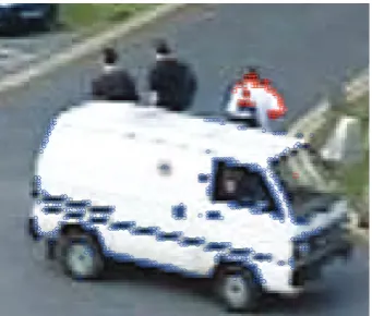
The tracking procedure which is an implementation of the sequential procedure described inSection 4.2is described inAlgorithm 1. The collaborative tacking procedure will be explained discussing a step of the algorithm using a sequence taken from the PETS2001 dataset. Figure 5(a) shows the tracking problem. There is a man that is partially occluded by a van. At the first step, as explained inTable 1, the single object tracking algorithm is used for both the van and the man as if they were alone in the scene. The likelihood is shown inFigure 6. In Figures6and7, the winner maximum
O(0)=∅
fori=0 toL−1
R=Ntj\
O(0)· · ·O(i) forl=1 toL−i
Winner maximum estimation for trackerR(l) Corner classification for trackerS(l)
Q(l)=sizeSl G
/sizeXls,t−1
end
O(i)=R
argmax
k
Q(k)
Assign the winner maximum position toXOp,(ti)
Assign the corners inSG, SS, andSNofO(i) to the set of
observation ofO(i)
RemoveSGofO(i) from the scene
end
Algorithm1: Position estimation in collaborative tracking.
is plotted as a square, while the far maxima (that are a symptom of multimodality) are plotted as circles. To maintain the figures clear, the close maxima that are near the winner maximum are not plotted because they do not give information about the multimodality of the distribution. Since always 4 maxima are extracted, considering that one of them is the winner, in the figures where less than 4 maxima are plotted, it should be considered that k (wherek = 3-number of far maxima) near maxima are extracted but not plotted. As it is possible to see, while the voting space of the van inFigure 6(b)is mainly monomodal (only one far maximum is extracted), the voting space inFigure 6(a)that corresponds to the occluded man is multimodal, because also the corners belonging to the van participate in the voting.
(a) (b) (c)
Figure5: (a) Problem formulation. (b) Van’s good corners at first step. (c) Man’s good corners at first step.
Table1: Position estimation in collaborative tracking.
Sequence 1 Sequence 2 Sequence 3
108 frames resolution 85 frames resolution 101 frames resolution
720×576 320×240 768×576
Collaborative with feature
classification Successful Successful Successful
Noncollaborative with fea-ture classification
Fails at the interac-tion between tracked targets
Fails for model cor-ruption at frame 80
Fails at the interac-tion between tracked targets
Collaborative without
fea-ture classification Successful Fails Fails after few frames
ID is assigned to O(1). Since the van is perfectly visible, it is possible to estimate its positionXOp,(1)t as if it were alone in the scene; the corners belonging to SG, SS, and SN are assigned as the observations that belong to the trackerO(1) (see Figure 5(b)); the corners belonging toSG are removed from the scene, and the procedure is iterated. In this way only the corners that do not belong to the van (Figure 5(c)) are used for the estimation of the position of the man. As it is possible to see fromFigure 7(a)the voting space of the man, after the corners of the van have been removed, is monomodal (the number of far maxima is decreased from 3 as inFigure 6(a)to 1) and its maximum corresponds to the position of man in the image.
The collaborative shape estimation is a greedy method that solves at the same time the position estimation and the observation assignment. As all the sequential methods, it is in theory prone to accumulation of errors (i.e., a wrong estimation of one tracker can generate an unrecoverable failure in the tracking process of all the trackers that are estimated after it). Our method is however quite robust.
The proposed method can make essentially two kinds of errors:
(1) an error in the estimation order;
(2) an error in the estimated position of one or more trackers.
An error of kind 1 would damage the shape model but, due to the presence in the shape model of points with high persistency, the model would resist for some frames
to this kind of error. An error of kind 2 generates a displacement of the bounding box that can, in the shape updating process, damage the model. Since the search space (defined as the zone where the observations are extracted) in the collaborative modality is the union of the search regions of the single trackers, in case of collaboration, a displacement error can be recovered with more ease since the search region is larger.
4.4.2. Shape estimation
The shape estimation is realized in two steps: at first the a priori shape estimation with exclusion principle is realized, and then the estimation is corrected by using the observations. The a priori shape estimation does not allow an increase of persistency in more than a model point if they lie on the same absolute position. After this joint shape a priori estimation, the assignment of features is revised using the feature classification information in a collaborative way.
700 650
600 550
500
Voting space seen by 1
450 400 350
(a)
700 650
600 550
500
Voting space seen by 2
450 400 350
(b)
Figure6: Likelihood estimation at first step. (a) V(·) seen by the man’s tracker. (b) V(·) seen by the van’s tracker. The winner maximum is plotted as a square and the far maxima are plotted as circles.
700 650
600 550
500
Voting space seen by 1
450 400 350
(a)
700 650
600 550
500
Voting space seen by 2
450 400 350
(b)
Figure7: Likelihood estimation at second step. (a) V(·) seen by the man’s tracker. (b) V(·) seen by the van’s tracker. The winner maximum is plotted as a square and the far maxima are plotted as circles.
Figure8: Corners updated in the van’s and person’s models.
The rules defined inSection 4.3.2are implemented and the corners are assigned accordingly. The results of applying this method to the frame in Figure 5(a) are reported in
Figure 8 where the model points that had an increase in persistence, considering both the shape a priori estimation and the likelihood calculation are shown. As it is possible to see from the figure that each tracker was updated correctly (no model points were added or increased in persistence for
the man in the zone of the van and vice versa) demonstrating a correct feature classification.
5. EXPERIMENTAL RESULTS
The proposed method has been evaluated on a number of different sequences.
This section illustrates and evaluates the performances by discussing some examples that show the benefits of the collaborative approach and by proposing some qualitative and quantitative results. The complete sequences presented in this paper are available at our website [17].
As a methodological approach for the comparison, considering that this paper focuses on the classification of the features in the scene and on their use for collaborative tracking, mainly results related to occlusion situations will be presented.
5.1. Comparison with single-tracking methodology
At first, the results of the new collaborative approach have been compared to the results obtained using the single tracking methodology and to an approach of collaborative tracking that does not use classification information [18].
Frame 10 (a)
Frame 27 (b)
Frame 40 (c)
Frame 48 (d)
(e) (f) (g) (h)
Figure9: Sequence 1. Tracking results. Upper row: collaborative approach. Lower row: noncollaborative approach.
Frame 27 (a)
Frame 35 (b)
Figure10: Sequence 1. Shape-updating results during collaboration.
interact with severe occlusion. In the sequence, two persons coming from the left of the scene interact constantly with partial occlusion; another person with a trolley coming from the right walks between the two persons occluding one of them and being occluded by the other. The persons wear dark clothes, and hence it is difficult to extract corners when there is an overlap between the silhouettes. InFigure 9, the results obtained using three independent trackers (bottom row) and those obtained using the proposed collaborative method (upper row) are compared.
As it is possible to see, one of the independent trackers looses track because it uses for shape-model updating the corners belonging to the other tracker. In the figure, the convex hull ofXs,tcentred onXp,t is plotted using a dashed line while the bounding box is plotted using a solid line. As it is possible to see by comparing the estimated shapes, the shape estimation using the collaborative methodology is more accurate than the independent one.
InFigure 10, the updated corners are plotted on top of the image to show which corners are updated and by which tracker (the background corners are not plotted for ease of visualization). As it is possible to see, each model is updated
using only the corners that belong to the tracked object and not to other objects.
At frame 35, it is possible to see that the shape model of the man coming from the right is correctly updated at its left and right sides, while in the centre, due to the presence of the foreground person, the algorithm chooses not to update the model.
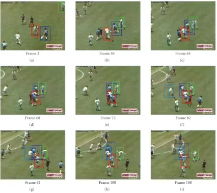
The next example (Sequence 2) is a sequence taken from a famous soccer sequence in which the tracked objects are involved in constant self occlusion. The quality of the images is low due to compression artefacts. In Figure 11, some frames of the sequence are displayed. As it is possible to see, the tracking process is successful and the shape is updated correctly.Figure 12(a)contains the results obtained with the proposed approach while Figure 12(b)contains the results of the noncollaborative approach. As it is possible to see, the convex hull ofXs,t is accurate in case of collaboration. If the trackers do not share information, they include in their model also corners of other objects (see the central object in
Frame 2 (a)
Frame 55 (b)
Frame 63 (c)
Frame 68 (d)
Frame 72 (e)
Frame 82 (f)
Frame 92 (g)
Frame 100 (h)
Frame 108 (i) Figure11: Sequence 2. Collaborative approach with feature classification results.
(a) (b)
Figure12: Sequence 2. Comparison between (a) collaborative and (b) noncollaborative approaches.
approach that does not use feature classification (Figure 13
right column) is reported. As it is possible to see, the feature classification allows the rejection of clutter (some soccer players are not tracked and are therefore to be considered
clutter). Using a tracker without feature classification, cor-ners that belong to clutter are used for shape estimation; and for this reason, tracking will fail in few frames (third row of
Figure 13).
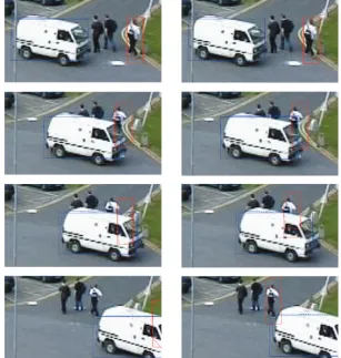
Another example (Sequence 3) is the sequence that was used to discuss the collaborative position and shape updating inSection 4.4. InFigure 14left column, the results obtained using the noncollaborative approach are reported. The noncollaborative approach fails because the corners of the van are included in the model of the person and its model is corrupted. In the collaborative approach, the shape is correctly estimated as shown inFigure 14right column.
InTable 1, a summary of the results is reported.
5.2. Tracking results on long sequences
Figure13: Sequence 2. Comparison between collaborative approach with feature classification (central column) and collaborative approach without feature classification (right column).
considered as one error since the two trackers which failed were collaborating) that occur after 500 frames from the initialization of the trackers. During these 500 frames, the trackers experienced a constant interaction between them and with another tracker in a cluttered background. The low-error rate demonstrates the capabilities of the algorithm also on long sequences. Sequences 4 and 5 are available at our website [17].
5.3. Quantitative-shape estimation evaluation
To discuss the shape-updating process and the benefits of collaboration from a quantitative point of view, some results that are related to Sequence 2 are provided in Figures 15
and 16. A particularly interesting measure of the benefits of the collaborative approach with feature classification is presented inFigure 15. The convex hull of the target labeled as 1 inFigure 11has been manually extracted. By counting the number of model points that, due to the updating process, have an increased persistence and that are outside this manually extracted convex hull and which therefore belong to clutter or other objects, it is possible to have a
measure of the correctness of the shape update process. From the graph, it is clear that from frames 3 to 10 and particularly after frame 55 (the heavy occlusion of Figure 12), many more model points are updated or added outside the target’s convex hull by the noncollaborative approach. This is due to the fact the algorithm inserted model points using the evidence of other objects. This errors lead to a failure after few frames (for this reason, the noncollaborative approach graph ends at frame number 80).
Figure14: Sequence 3. Comparison between noncollaborative (left column) and collaborative approaches (right column).
Table2: Tracking results.
PETS2006 name Number of frames Number of objects Short-term interaction Long-term interaction Failures
Sequence 4 S3-T7-A 2271 19 8 3 0
Sequence 5 S6-T3-H 2800 14 5 2 2
120 100 80
60 40 20 0
Frame number Noncollaborative approach Collaborative approach 0
200 400 600 800 1000 1200 1400 1600 1800
M
o
del
p
oints
w
ith
incr
eased
persist
enc
e
Figure15: Sequence 2. Number of model points with increased persistence outside the manual extracted convex hull of the target.
proof of the ability of the collaborative approach with feature collaboration to adapt to the scene, even in case of heavy interaction between the tracked objects.
5.4. Sensitivity to background clutter
To evaluate the performances of the algorithm in cluttered situations, three experiments have been set up. A sequence (Sequence 6) that is correctly tracked in normal condi-tions has been selected (the tracking results are shown in