Analysis of the Properties of a Third Order Convergence Numerical Method Derived via the Transcendental Function of Exponential Form

http://www.sciencepublishinggroup.com/j/ijamtp doi: 10.11648/j.ijamtp.20190504.11

ISSN: 2575-5919 (Print); ISSN: 2575-5927 (Online)

Analysis of the Properties of a Third Order Convergence

Numerical Method Derived via the Transcendental Function

of Exponential Form

Sunday Emmanuel Fadugba

*

, Jethro Olorunfemi Idowu

Department of Mathematics, Faculty of Science, Ekiti State University, Ado Ekiti, Nigeria

Email address:

*

Corresponding author

To cite this article:

Sunday Emmanuel Fadugba, Jethro Olorunfemi Idowu. Analysis of the Properties of a Third Order Convergence Numerical Method Derived Via the Transcendental Function of Exponential Form. International Journal of Applied Mathematics and Theoretical Physics. Special Issue: Computational Mathematics. Vol. 5, No. 4, 2019, pp. 97-103. doi: 10.11648/j.ijamtp.20190504.11

Received: September 14, 2019; Accepted: October 18, 2019; Published: November 4, 2019

Abstract:

This paper proposes a new numerical method for the solution of the Initial Value Problems (IVPs) of first order ordinary differential equations. The new scheme has been derived via the transcendental function of exponential type. The analysis of the properties of the method such as local truncation error, order of accuracy, consistency, stability and convergence were investigated. Two illustrative examples/test problems were solved successfully to test the accuracy, performance and suitability of the method in terms of the absolute relative errors computed at the final nodal point of the associated integration interval via MATLAB codes. It is observed that the method is found to be of third order convergence, consistent and stable. The numerical results obtained via the method agree with the exact solution. Moreover, it is also observed that the method is an improvement on Fadugba-Falodun scheme. Hence, the proposed numerical method is a good approach for solving the IVPs of various nature and characteristics in diverse areas of Ordinary Differential Equations (ODEs).

Keywords:

Accuracy, Consistency, Convergence, Initial Value Problem, Local Truncation Error, Order of Accuracy, Region of Stability, Stability

1. Introduction

Many scientific and technological problems in natural and engineering are modeled mathematically by both partial and ordinary differential equations. For instance, in physics heat flow and wave propagation phenomenon are well defined by partial differential equations. Hence, there are various natural and physical phenomena in which differential equations play a vital role. In as many as possible engineering and scientific fields, it is a known fact that several mathematical models emanating from the real life situations cannot be solved explicitly, one has to compromise at numerical approximate solutions of the models achievable by various numerical techniques of different characteristics. One numerical technique may differ from the other in terms of its convergence, order of accuracy, local errors, stability, efficiency and computational complexity. Development of numerical methods for the solution of initial value problems

in ordinary differential equations has attracted the attention of many researchers in recent years. There are numerous methods that produce numerical approximations to solution of initial value problems in ordinary differential equations such as Euler’s method which was the oldest and simplest method originated by Leonhard Euler in 1768, Improved Euler method, Runge Kutta methods described by Carl Runge and Martin Kutta in 1895 and 1905 respectively.

Many authors have derived new numerical integration methods, giving better results than a few of the available ones in some literature [1-15], just to mention a few.

2. Derivation of the Proposed Numerical

Method

This section presents the derivation of the proposed numerical method via the transcendental function of exponential type of the form

= ∑ + (1)

For the solution of the initial value problem;

= , , = , , ,

−∞ < < ∞ (2) From equation (1), we have

= + + + (3)

Where , , are undetermined constants.

Consider the integration interval of [a, b] which can be partitioned as follows

= < < < ⋯ < "= (4) The step length, h is defined as

ℎ = $ %

& or ) *

& (5)

Alternatively,

ℎ = "+ − ", = 0,1,2, … 0 − 1 (6)

Expanding equation (3) at = _", yields

" = + "+ "+ $ (7)

Similarly, for = _"+ , one gets

"+ = + "+ + "+ + $12 (8)

Let,

" = " (9)

" = " (10)

" = " (11)

Differentiating (7) with respect to _" yields

" = + 2 "− $ (12)

Differentiating (12) with respect to _" yields

" = 2 + $ (13)

Similarly, the third derivative of _" gives

" = − $ (14)

Using (9), (10), (11), (12), (13) and (14), one obtains

" = + 2 "− $ = " (15)

" = 2 + $= " (16)

" = − $ = " (17)

Therefore,

+ 2 "− $= " (18)

2 + $ _{= " (19)} − $ = _{" (20)}

From equation (20), we obtain

= 3$4

567$ = − $ " (21)

Using (21) in (19), yields

2 + 8− $ _{" 9} $_{= "} 2 − " = "

2 = " + "

= (_" + _" ) (22)

Substituting (21) and (22) into (18), yields

+ 2 :1_{2 8}" + " 9; "+ " = "

+ 8 " + " 9 "+ " = "

= "− 8 " + " 9 "− " (23)

The undetermined constant , are given by

(23), (22), and (21) respectively.

We defined the mesh point _" as

"= + ℎ (24)

Also

"+ = + + 1 ℎ (25)

This implies that

"+ − "= + 1 ℎ − ℎ = ℎ + ℎ − ℎ = ℎ

Therefore,

"+ − "= ℎ (26)

In this paper we set = 0,

Thus (24) and (25) become

"= ℎ (27)

"+ = + 1 ℎ (28)

respectively,

Subtracting (7) from (8) yields

"+ − " = − + "+ − "

= "+ − " + "+ − " + $12 $ (29) But from (26), we have

"+ − "= ℎ

Also,

"+ − "= + 1 ℎ − ℎ

= + 2 + 1 ℎ − ℎ = ℎ + ℎ 2 + 1 − ℎ

= 2 + 1 ℎ (30) Substituting (26) and (30) into (29), yields

"+ − " = ℎ + 2 + 1 ℎ

+ "+ <₋ "<

= ℎ + 2 + 1 ℎ + "< <_{− 1 (31)}

From equation (21), with _"= ℎ

= − "<

" (32)

Also,

= "− 8" + " 9 ℎ − " (33)

Substituting (22), (32) and (33) into (31) yields

"+ − " = 8 "− 8" + " 9 ℎ − " 9ℎ +1_{2 8}" + " 9 2n + 1 ℎ + 8− "< " 98 "< <− 1 9

= ℎ"− ℎ 8 " + " 9 − ℎ" +1_{2 8}" + " 9 2n + 1 ℎ − " <− 1

= ℎ"− ℎ " − ℎ " − ℎ " + "_{2 2 + 1 ℎ +} "_{2 2 + 1 ℎ −} " <− 1

= ℎ"+ ℎ >− " − " + "_{2 2 + 1 +} "_{2 2 + 1 ? +} " 1 − <− ℎ

"+ − " = ℎ "+ ℎ @− " − " + " + "_{2 +} " + "_{2 A}

+ 1 − <_{− ℎ} "

"+ − " = ℎ "+<

4

8" + " 9 + 1 − <− ℎ " (34)

Using the fact that

"+ − " ≡ "+ − " (35)

Thus,

"+ − "= ℎ"+< 4

C" + " D + 1 − <− ℎ " (36)

The newly derived numerical method via the

transcendental function of exponential type for the solution of the initial value problem in ordinary differential equations is given by

"+ = "+ ℎ"+< 4

C" + " D + 1 − <− ℎ " (37)

Remarks 2.1

Equation (37) is called the proposed numerical method. Equation (37) is derived from transcendental function of exponential type.

Equation (37) is an improvement of Fadugba-Falodun scheme given by

"+ = "+ ℎ"+ 8ℎ + <− 1 9 "

3. Analysis of the Properties of the

Method

This section presents the analysis of the properties of the method as follows:

3.1. Local Truncation Error Analysis

The analysis of local truncation error indeed decides the order of convergence for any numerical technique designed to solve the initial value problem in ODEs. In order to check the order of the technique, we subtract the algorithm of the numerical technique (37) from the well-known Taylor’s

series expansion for in powers of h which has been

described below.

Consider the Taylor’s series expansion of the form

"+ ℎ = " + ℎ +<

4

! +

<F

! +

<G

H! + O ℎJ (38)

The newly derived numerical integration method of the form

"+ = "+ 1 − < " + ℎ "− " +<

4

The local truncation error denoted by LTE is defined as

LTE = "+ ℎ − "+ = " + ℎ +ℎ_2! +ℎ_3! +ℎ H

4! + O ℎJ

− @ "+ 1 − < " + ℎ8"− " 9 +ℎ_{2 8}" + " 9A

= " + ℎ +<

4

! +

<F

! +

<G

H! − : "+ 1 − < " + ℎ8"− " 9 + <4

8" + " 9; + O ℎJ (40)

Replacing the term < by Maclaurin’s series, one obtains

LTE = " + ℎ +ℎ_2! +ℎ_3! +ℎ H

4!

− > "+ @1 − :1 − ℎ +ℎ_{2! −}ℎ_{3! +}ℎ H

4! + ⋯ ;A " + ℎ8"− " 9 +ℎ_{2 8}" + " 9? + O ℎJ

LTE = " + ℎ +ℎ_2! +ℎ_3! +ℎ H

4!

− : "+ :1 − 1 + ℎ −ℎ_{2! +}ℎ_{3! −}ℎ H

4! + ⋯ ; " + ℎ "− ℎ " +ℎ₂ " +ℎ₂ " ; + O ℎJ

= " + ℎ +ℎ_2! +ℎ_3! +ℎ

H

4!

− : "+ ℎ " −ℎ_2! " +ℎ_3! " −ℎ H

4! " + ⋯ + ℎ"− ℎ " +ℎ₂ " +ℎ₂ " ; + O ℎJ

LTE = " + ℎ +<

4

! +

<F

! +

<G

H! − C "+ ℎ"+ <4

" +<

F

! " − <G

H! " D + O ℎJ (41)

Under local assumption, the term up to ℎ have been

cancelled and we are left with the following expression

LTE =_{4! 8ℎ}1 H _{− ℎ}H

" 9 + O ℎJ

LTE =<_HG8 − " 9 + O ℎJ (42)

Thus, the leading term of the local truncation error

involve ℎH which confirms the third order accuracy of the

numerical integration method given by (37). Hence, the proposed numerical integration has the convergence of the third order.

3.2. Consistency Analysis of the Method

For a numerical method to be consistence, it is important for the truncation error to be zero when the step size, h, gets smaller and ultimately reaches to zero. Among many, one of the ways of analyzing consistency of a numerical technique is to check that whether

lim<→ TUV_< = 0 (43)

From (42), we have that

lim<→ < G

HC − " D ℎW = lim<→ <F

HC − " D = 0 (44)

Equation (43) has been established. From (44), it is seen/observed that the proposed numerical integration method has consistency property. Further, it is also known that any technique having order of accuracy greater than zero is considered to be consistent. Based on this fact, consistency of the proposed technique can safely be claimed since third order accuracy of the proposed technique has already been proved in the previous section.

3.3. Stability Analysis of the Scheme

Numerical methods are said to be numerically stable if they are capable of damping out the small fluctuations carried out in input data. The notion of stability may be taken in different contexts: it may be associated with the specific

numerical technique used, or the step size, h used in

numerical computation or with the particular problem being solved.

For stability analysis of the proposed numerical integration method (37), one of the popular ways is to apply it to the problem

= −X , 0 = 1 (45) which has the theoretical solution of the form

Where λ is in general, a complex constant.

For the integration interval _", _"+ , where # _"+

"; the exact solution at the point "+ is

"+ Y $12 Y $. Y<

"+ " . Y< (47)

Where h is defined as _{"+ "} # . The numerical

approximation obtained using the proposed technique gives

"+ " # X " #_{2! X} " #_{3! X} "

"+ "C1 X# Y

4_<4

! YF_<F

! D (48)

Let

B 1 X# Y4<_!4 YF<_!F (49)

Then

"+ B " (50)

Comparing (47) and (50), this shows that the factor B is

merely an approximation for the factor Y< in the exact

solution. Truly, the factor B is the four-term approximation

for the maclaurin’s series for Y< for small λh. The error

growth factor B can be controlled by ‖B‖ 1, so that the

errors may not magnify. Thus, the stability of the proposed numerical integration method requires that

^1 X# Y4<_!4 YF<_!F^ 1 (51)

Setting z = λh, then (51) becomes

^1 X_ `4<sub>!</sub> `F_!^ 1 (52)

By means of (52), the stability region of the scheme is plotted in the Figure 1. Hence, the proposed numerical integration method (37) is found to be conditionally stable with the region of linear stability given below.

Remark 3.1

The proposed numerical method is said to have convergence for any given, well-posed initial value problem since it satisfies both consistency and stability properties as discussed above.

3.4. Algorithm of the New Numerical Method

An approximate solution to the initial value problem

, , , ∈ b, ,

At the equal space points at , , , … , _" is given by

"+ " # " #_{2 8}" " 9 1 < # "

"+ 1 #, for 0 1 0 1

Where

# "+ " ) *_&

and are given initial conditions.

Figure 1. Stability region (shaded) for the numerical integration method.

4. Illustrative Examples

It is usually necessary to demonstrate the suitability and applicability of the newly developed method. In this course, the algorithm of the scheme has been successfully translated into MATLAB programming language and implemented with a problem emanated from real life situations. The performance of the method has been checked by comparing its accuracy and efficiency with the exact solution. The efficiency was determined from the number of iterations counts and number of functions evaluations per step while the accuracy is determined by the size of the discretization error estimated from the difference between the exact solution and the numerical approximations.

Test Problem 1

Consider the initial value problem of the form

, (0) 1, 0 1, 0.1

y′ =y y = ≤ ≤x h= (53)

Whose exact solution is obtained as:

( ) x

y x =e (54)

With different values of the step length

0.1,0.01,0.001,0.0001

h

=

.

Table 1. The comparative results analyzes of the Fadugba Scheme 'YN' and the exact solution 'YXN' with different values of 'h'.

'h' 'XN' 'YN' 'YXN' 'EN'

0.1 1.0000000000 2.7180768002 2.7182818285 0.0002050283 0.01 1.0000000000 2.7182816042 2.7182818285 0.0000002243 0.001 1.0000000000 2.7182818282 2.7182818285 0.0000000002 0.0001 1.0000000000 2.7182818285 2.7182818285 0.0000000000

Figure 2. The comparative results analyses using Table 1.

Figure 3. Error incurred in the numerical method.

Test Problem 2

Let us assume that a colony of 1000 bacteria is multiplying

at the rate of r 0.8 per hour per individual (that is; an

individual produces an average of 0.8 off spring every hour).

How many bacteria are there after 1 hour? It is assumed that

the colony grows continuously and without restriction. It is possible to model this growth with a differential equation of first order of the form:

e& f

ef g0 h (55)

with initial condition

0 0 1000 (56)

Equations (55) and (56) become

e& f

ef g0 h , 0 0 1000, g 0.8 (57)

where 0 h is the population size at time h. The exact

solution to (55) subject to (56) is obtained as

0 h 1000e .jk ₍₅₈₎

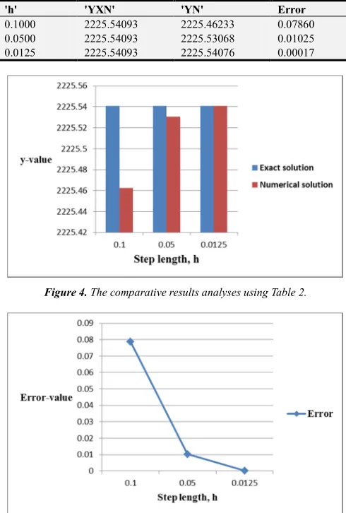
The comparative results analyses of the method ‘YN’ and the exact solution 'YXN' were shown in Table 2 below.

Table 2. The comparative results analyses of the method 'YN' and the exact solution 'YXN'.

'h' 'YXN' 'YN' Error

0.1000 2225.54093 2225.46233 0.07860 0.0500 2225.54093 2225.53068 0.01025 0.0125 2225.54093 2225.54076 0.00017

Figure 4. The comparative results analyses using Table 2.

Figure 5. Error incurred in the numerical method.

5. Concluding Remarks

In this paper, a new numerical method has been successfully developed via a transcendental interpolating function of exponential type for the solution of initial value problems of first order. The proposed numerical method is found to be of third order convergence, consistent and stable. Two illustrative examples have been solved to test the performance of the technique in terms of the absolute relative errors computed at the final nodal point of the associated

integration interval via MATLAB codes. It is observed from

Figure 2 that the value of the method coincides with the exact solution for h = 0.0001. It is clearly seen from Table 2 that as the computation progresses with different step lengths, the error incurred via the proposed numerical method reduces. Hence, proposed numerical method can be considered a good candidate to be included in the family of linear explicit numerical techniques employed for the purpose of finding numerical solutions of various physical and natural systems.

Some extensions and modifications of the methodology can be explored by further research. A natural extension is the applications of the proposed numerical method for the solution of some special initial value problems differential equations with point of singularity.

References

[1] N. Ahmad, S. Charan, and V. P. Singh, Study of numerical accuracy of Runge-Kutta second, third and fourth order method, 2015.

[2] Y. Ansari, A. Shaikh, and S. Qureshi. Error bounds for a numerical scheme with reduced slope evaluations, J. Appl. Environ. Biol. Sci, 8 (7), 2018.

[3] J. C. Butcher, Numerical methods for ordinary differential equation, West Sussex: John Wiley & Sons Ltd, 2003. [4] M. E. Davis, Numerical methods and modeling for chemical

engineers, Courier Corporation, 2013.

[5] S. E. Fadugba, Numerical technique via interpolating function for solving second order ordinary differential equations, Journal of Mathematics and Statistics, 1: 1-6, 2019.

[6] S. E. Fadugba and A. O. Ajayi, Comparative study of a new scheme and some existing methods for the solution of initial value problems in ordinary differential equations, International Journal of Engineering and Future Technology, 14: 47-56, 2017.

[7] S. Fadugba and B. Falodun, Development of a new one-step scheme for the solution of initial value problem (ivp) in ordinary differential equations, International Journal of Theoretical and Applied Mathematics, 3: 58–63, 2017. [8] S. E. Fadugba and J. T. Okunlola, Performance measure of a

new one-step numerical technique via interpolating function for the solution of initial value problem of first order differential equation, World Scientific News, 90: 77–87, 2017. [9] S. E. Fadugba and T. E. Olaosebikan, Comparative study of a

class of one-step methods for the numerical solution of some initial value problems in ordinary differential equations, Research Journal of Mathematics and Computer Science, 2: 1-11, 2018, DOI: 10.28933/rjmcs-2017-12-1801.

[10] J. D. Lambert, Numerical methods for ordinary differential systems: the initial value problem, John Wiley & Sons, Inc., New York, 1991.

[11] R. B. Ogunrinde and S. E. Fadugba, Development of the New Scheme for the solution of Initial Value Problems in Ordinary Differential Equations, International Organization of Scientific Research Journal of Mathematics (IOSRJM), 2: 24-29, 2012. [12] J. D. Lambert, Computational methods in ordinary differential

equations, John Wiley & Sons Inc, 1973.

[13] S. E. Fadugba and S. Qureshi, Convergent numerical method using transcendental function of exponential type to solve continuous dynamical systems, Punjab University Journal of Mathematics, 51: 45-56, 2019.

[14] J. C. Butcher, Numerical methods for ordinary differential equations, John Wiley & Sons, 2016.