R E S E A R C H
Open Access
Parallelization of the optical flow computation
in sequences from moving cameras
Antonio Garcia-Dopico
*, José Luis Pedraza, Manuel Nieto, Antonio Pérez, Santiago Rodríguez
and Juan Navas
Abstract
This paper presents a flexible and scalable approach to the parallelization of the computation of optical flow. This approach is based on data parallel distribution. Images are divided into several subimages processed by a software pipeline while respecting dependencies between computation stages. The parallelization has been implemented in three different infrastructures: shared, distributed memory, and hybrid to show its conceptual flexibility and scalability. A significant improvement in performance was obtained in all three cases. These versions have been used to
compute the optical flow of video sequences taken in adverse conditions, with a moving camera and natural-light conditions, on board a conventional vehicle traveling on public roads. The parallelization adopted has been developed from the analysis of dependencies presented by the well-known Lucas-Kanade algorithm, using a sequential version developed at the University of Porto as the starting point.
Keywords: Optical flow; Parallelization; Cluster; MPI; Threads; Onboard camera
1 Introduction
Optical flow is an image analysis technique used to detect motion in video sequences. The detection can be per-formed in real time while images are being captured, or afterwards, when they are already stored in video format. Therefore, the optical flow works on an image sequence. For each image of the sequence, it generates a vector at each image pixel representing the apparent motion in the corresponding sampling period.
To determine the apparent motion of objects in an image, the information generated by the optical flow and by a separate process that identifies the different objects can be used. However, the apparent simplicity by which the human eye interprets movement in a three-dimensional space represents a highly complex task when trying to emulate it with computers - even in the case of a single motion.
The movement represented by the optical flow is con-sidered an apparent movement since, in fact, the set of vectors generated is obtained from a two-dimensional image arising from projecting the real image
(three-*Correspondence: [email protected]
DATSI, Facultad de Informática, Universidad Politécnica de Madrid Boadilla del Monte, Madrid 28660, Spain
dimensional) on the plane of the camera. Moreover, optical flow computation techniques are based on ana-lyzing the brightness variations of each pixel, making it impossible to distinguish between true and apparent motion. In fact, it is not possible to determine whether a velocity vector is obtained due to an actual motion of an object or a movement of the camera that has cap-tured the image or a variation of luminosity due to some environmental condition such as reflections or shadows.
Technically, optical flow computation is based on assumptions rarely observed in real cases, but they can be partially met and so be considered as valid approx-imations. These are, as described by Beauchemin and Barron [1], (a) uniform illumination, (b) surfaces with Lambertian reflectance, and (c) movement limited to the plane of the image. Since most applications rarely meet the aforementioned conditions, it is considered that the method is approximate and that it does not allow the reconstruction of the original movement produced in the three-dimensional scene. However, in many occasions, the optical flow allows obtaining valid approximations of the movement being actually recorded.
Determining optical flow is a subject that has been studied by means of computers for several decades, and it has been employed in applications, such as (a)
dimensional image segmentation [2], (b) support for nav-igation of autonomous robots or, in general, the detection of obstacles to avoid collisions [3-6], (c) synchronization and/or ‘matching’ of video scenes [7], and (d) fluid dynam-ics analysis [8]. In any case, the problem is computation-ally very complex, so most of the proposed solutions are based on strong simplifications adapted to the technology available at the time or to the specific applications they intend to solve. In some cases, the size of the images is so small that can hardly represent a real-life scene [9-12]. In other cases, determining parameters in the generation of optical flow such as the light source (source, intensity, variation, etc.) or the motion of objects within the scene are restricted [13-15]. Except for some recent articles normally associated with the movement of conventional vehicles [16,17], mobile robots [18,19], and handheld cam-eras [20,21], the majority of papers describe systems in which the variation of the scene is limited. This limitation is determined because they work with images with a static background and taken with a static camera.
This article focuses on the parallelization of an optical flow computing system based on the well-known Lucas-Kanade algorithm [22,23]. The system is applied to an environment which is particularly hostile in terms of opti-cal flow computation and has rarely been described by other authors [19]. It aims to determine the motion visu-ally perceived by the driver of a conventional vehicle through roads or streets under real conditions: with real traffic and moving at speeds ranging from a few kilome-ters per hour to 120 km/h. Not only do these conditions rule out the parameter restrictions applied to other sys-tems (i.e., regarding image size, controlled light sources), but they in fact all act simultaneously in generating the optical flow. Thus, image resolution must be sufficient (in the order of 500 × 300 pixels) to capture multiple objects of different sizes. Also, the camera moves with the car because it is located inside it. Finally, the light con-ditions are natural and highly variable. Hence, applying the restriction used in other systems is largely impossible. Moreover, obtaining the optical flow directly during the driving session requires the analysis of medium- or high-resolution video sequences in real time which requires significant computing capacity. This aspect may be exac-erbated when working with large volumes of information coming from complete sessions previously stored, for which the corresponding optical flow has to be obtained. In these cases, it may be necessary to work faster than real time to obtain the optical flow of all the stored video in a reasonable amount of time.
The requirements described above prompted the authors to choose a well-tested and verified algorithm, providing the required accuracy. Considering all these factors and in accordance with the analysis of different algorithms and their benefits [24,25], the Lucas-Kanade
method, which has good quality results with moderate computational cost, has been chosen. Specifically, the sequential implementation by Correia at the Biomedical
Engineering Institute, Engineering School of the
University of Porto [26,27] has been used.
Other authors have addressed the parallelization of opti-cal flow computing systems. However, in most of the cases, the chosen solutions require specific hardware, such as those based on FPGA, on which there is abun-dant literature [5,28]. By contrast, this article presents three implementations of a parallelization approach which relies solely on low-cost general-purpose computers. The implemented versions are all based on the sequential implementation from Correia [26] and are the follow-ing: (a) distributed, supported by a cluster of computers; (b) parallel, supported by a shared memory multiproces-sor; (c) hybrid, supported by a cluster of multiprocessors. The paper describes the characteristics of the three par-allelizations mentioned and analyzes them from the point of view of their performance, because all of them per-form the same computations as the sequential algorithm and thus produce the same results. The specific details of the sequential implementation of the Lucas-Kanade algorithm and the results obtained can be found in [26,27].
2 Parallelization of the optical flow
There is a variety of algorithms to perform the computa-tion of the optical flow. Most of them are based on the classical and well-established algorithms analyzed in [24], which usually have an initial premise for their correct operation, the assumption that the illumination intensity is constant along the analyzed sequence.
Each algorithm presents some advantages and disadvan-tages; the main drawback of most of the algorithms is their high computational and memory costs. Some of them try to reduce these costs by sacrificing accuracy of results, i.e., they balance the cost of the algorithm against the level of accuracy.
There have been many alternatives and they have evolved along with the technology. In some cases, SIMD processor arrays with specific chips, either existing [36] or designed ad hoc for the computation of optical flow [13,17,37-39], have been used. General-purpose MIMD as the connection machine [40,41], networks of transputers [42], or cellular neural networks [43,44] were also used in the past.
In recent years, there have also been many imple-mentations based on FPGA [5,15,28,45-48] and graphic processor units (GPU) [6,8,49-51]. The results of a com-parative study of both technologies for real-time optical flow computation are presented in [52]. They conclude that both have similar performance, although their FPGA implementation took much longer to develop.
Some of the above methods for computing optical flow can be highlighted since they are based on the same Lucas-Kanade method used in this paper or their application appears to be similar to that described in this paper.
A system for driving assistance is presented in [17]. It detects vehicles approaching from behind and alerts the driver when performing lane change maneuvers. The sys-tem is based on images taken by a camera located in the rear of a vehicle circulating through cities and high-ways, i.e., under the same hostile conditions as our system. However, their model is simpler because it is limited to detecting large objects near the camera and moving in the same direction and sense. Their method is based on the determination of the vanishing point of flow from the lane mark lines and calculating the optical flow along straight lines drawn from the vanishing point. The optical flow is computed by a block-matching method using SAD (sum of absolute differences). The entire system is based on a special purpose SIMD processor called IMAPCAR imple-mented in a single CMOS chip that includes an array of 1×128 8-b VLIW RISC processing elements. It processes
256 × 240 pixel images at 30 fps. Their experimental
results show 98% detection of overtaking vehicles, with no false positives, during a 30-min session circulating on a motorway in wet weather. A real-time implementation of the Lucas-Kanade algorithm on the graphics proces-sor MaxVideo200 is presented in [51]. Due to hardware limitations, some of the calculations are performed on 8- and 16-b integer. Consequently, the results obtained are substantially worse than those obtained by Barron et al. for the same Lucas-Kanade method. In terms of real-time
performance, they are able to process 252 × 316 pixel
images in 47.8 ms, equivalent to a throughput of 21 fps. Another implementation of the Lucas-Kanade algo-rithm is presented in [28], this time based on FPGA. Their method is based on the use of high-performance cam-eras that capture high-speed video streams, e.g., 90 fps. Using this technology, they are able to reduce the motion of objects in successive frames. Additionally, variations in
light conditions are smaller due to the high frame rate, thus moving closer to meeting the constant illumination condition. In summary, a high frames-per-second rate allows simplifying the optical flow computation model and allows obtaining accurate results in real time. The division of the Lucas-Kanade algorithm into tasks is sim-ilar to that used in our method, although in [28], the pipeline is implemented using specific and reconfigurable FPGA hardware (Virtex II XC2V6000-4 Xilinx FPGA; Xilinx Inc., San Jose, CA, USA). Each pipeline stage is subdivided into simpler substages, resulting in over 70 substages using fixed point arithmetic for the most part. The throughput achieved is 1 pixel per clock cycle. Their system is capable of processing up to 170 fps with 800× 600 pixel images and, although its real-time performance should be measured relative to the acquisition frame rate, it appears to be significantly high for the current state of technology.
In recent years, cluster computing technology has spread to the extent of becoming the basic platform for parallel computing. In fact, today, most powerful super-computers are based on cluster computing [53]. However, it is unusual to find references to parallel optical flow algorithms designed to exploit the possibilities offered by clusters of processors to suit the size of the problems. In [54-56] some solutions are presented based on clusters and will be discussed in more detail.
A preliminary version of this paper [54] presents a par-allelization of the Lucas-Kanade algorithm applied to the computation of optical flow on video sequences taken from a moving vehicle in real traffic. These types of images present several sources of optical flow: road objects (lines, trees, houses, panels,...), other vehicles, and also heavily changing light conditions. The method described is based on dividing the Lucas-Kanade algorithm into several tasks that must be processed sequentially, each one using a dif-ferent number of images from the video sequence. These tasks are distributed among cluster nodes, balancing the load of their processors and establishing a data pipeline through which the images flow. The paper presents pre-liminary experimental results using a cluster of eight dual processor nodes, obtaining throughput values of 30
images per second with 502 ×288 pixel images and 10
fps with 720×576 pixel images. An interpolation method is also proposed to improve the quality of the optical flow obtained from video sequences taken by interlaced cameras.
The work by [55] presents a variational method based on the domain decomposition paradigm that minimizes the communication between processes and therefore is suitable for implementation in PC clusters. The
imple-mentation is based on dividing the problem inton× n
are analyzed: the Neumann-Neumann (NN) and the balancing-Neumann-Neumann (BNN) preconditioners which are applied to a pair of synthetic 2,000 × 2,000 pixel images. Their experimental results show that the NN approach provides better results than the non-parallel version on the basis of a decomposition into 5×5 sub-domains, obtaining increasing speed-up factors from 1.23 (5×5) to 3.67 (12×12) using between 25 and 144 pro-cessors. Processing time per frame goes from 10 down to 2 s.
The work in [56] addresses the optical flow calcula-tion with three-dimensional images by an extension of the Horn-Shunck model to three-dimensional. They study three different multigrid discretization schemes and com-pare them with the Gauss-Seidel method. They conclude that the multigrid method based on Garlekin discretiza-tion very significantly improves the results obtained using Gauss-Seidel method. They also perform a parallelization of the algorithm aimed at its execution in clusters and apply it to the calculation of three-dimensional motion of
the human heart using sequences of two 256 × 256 ×
256 and 512×512× 512 images taken by C-arm
com-puted tomography. Their method is based on subdividing the image into several three-dimensional subsets and pro-cessing each one in a different processor. The analyzed method is well suited to the proposed application because the image just include a single object (heart), with highly localized relative movements of expansion and contrac-tion. This fact, along with the uniformity of illumination, requires a very low communication overhead due to par-allelization. The speedup using 8, 12, and 16 processors is excellent: 7.8, 11.52, and 15.21, with an efficiency close to 1, but it starts to decrease when reaching 32 processors: 28.46. The experiments were performed on an eight-node quad-processor cluster.
3 The Lucas and Kanade algorithm
The Lucas and Kanade algorithm [22,23] takes a digital video as the only data source and computes the optical flow for the corresponding image sequence. The result is a sequence of two-dimensional arrays of optical flow vec-tors, with each array associated to an image of the original sequence and each vector associated to an image pixel. The algorithm analyzes the sequence frame by frame and performs several tasks. Some of them require some previous and some following images of the image being processed, so the optical flow is not computed for some of the images at the beginning and at the end of the sequence. The Lucas and Kanade algorithm computes the optical flow using a gradient based approach, so it calculates the spatiotemporal derivatives of intensity of the images. This method assumes that image intensity remains constant between frames of the sequence, a common assumption in many algorithms:
I(x,y,t)=I(x+ut,y+vt,t+t) (1)
This expression, using a Taylor series and assuming dif-ferentiability, can be expressed by the motion constraint equation:
Ixuδt+Iyvδt+Itδt=Ou2δt2,v2δt2 (2)
In a more compact form, takingδtas the time unit: ∇I(x,t)·v+It(x,t)=O
v2 (3)
where∇I(x,t)andIt(x,t)represent the spatial gradient
and temporal derivative of image brightness, respectively, andOv2indicates second order and above terms of the Taylor series expansion.
In this method, the image sequence is first convolved with a spatiotemporal Gaussian operator to eliminate noise and to smooth high contrasts that could lead to poor estimates of image derivatives. Then, according to the Barron et al. implementation, the spatiotemporal deriva-tivesIx,Iy, andItare computed with a four-point central
difference.
Finally, the two velocity components,v = vx,vy
, are obtained by a weighted least squares fit with local first-order constraints, assuming a constant model forvin each
spatial neighborhoodN and by minimizing
x∈N
W2(x)[∇I(x,t)·v+It(x,t)]2 (4)
whereW(x)denotes a window function that assigns more weight to the center. The solution is obtained from
v=
ATW2A
−1
ATW2b (5)
where, fornpointsxi∈Nat a single timet
– A=[∇I(x1), ...,∇I(xn)]T
– W=diag[W(x1), ...,W(xn)]
– b= −(It(x1), ...,It(xn))T
The productATW2Ais a 2×2 matrix given by:
ATW2A= W 2(x)I2
x(x)
W2(x)Ix(x)Iy(x)
W2(x)Iy(x)Ix(x) W2(x)Iy2(x)
(6)
where all the sums are taken over points in the neighbor-hoodN.
3.1 Implementation
In this section, the sequential implementation of the Lucas-Kanade algorithm proposed by Correia [26,27] is described because this implementation has been used as the starting point for the parallelization.
requires 25 pixels: the central pixel and 4σ (12) pixels on each side of this center pixel:
1 √
2πσe
−x2
2σ2 (7)
This one-dimensional symmetric Gaussian filter is applied three times, first on the temporal ‘t’ dimension, then on the spatial ‘X’ dimension, and finally on the spatial ‘Y’ dimension. Therefore, it needs 12 pixels on each side of the center pixel, and 4σ images (12) previous and next to the image being processed.
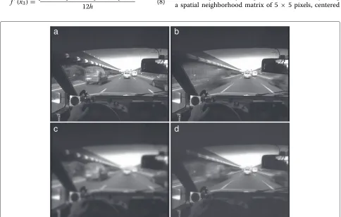
The result of applying the smoothing Gaussian filter on an image can be seen in Figure 1, which shows the original image, Figure 1a, and the three steps, the result for the temporal filter, Figure 1b, for the spatial filters, Figure 1c, and the global result, Figure 1d.
After smoothing, the next step of the Lucas and Kanade algorithm is to compute the spatiotemporal derivatives for the three dimensions:t,xandy(It,Ix, Iy). Using the
previously computed image, smoothed on t, X and Y,
and applying a numerical approximation, the derivatives (It,Ix,Iy) are computed separately. The method used is the 5-point central differences of Gregory-Newton and the derivative function for the central point is
f(x3)= f(x1)−
8f(x2)+8f (x4)−f(x5)
12h (8)
Takingh = 1 because the distance between two
con-secutive pixels is 1, the one-dimensional array to be used as convolution coefficient mask in the computation of the partial derivatives is obtained as follows:
1 12,
−8 12, 0,
8 12,
−1
12 (9)
Then, for each pixel of the image Itx,y, two
addi-tional pixels on each side of the central one are needed on each dimension. Two pixels to the right and left
Ix−t 2,y,Ix−t 1,y,Ixt,y,Ix+t 1,y,Ix+t 2,y are taken, as well as two
pixels above and below
Ixt,y−2,Itx,y−1,Ixt,y,Ixt,y+1,Ixt,y+2
, and one pixel in the two previous and in the two following images
Ixt−,y2,Ixt−,y1,Ixt,y,Ixt+,y1,Ixt+,y2
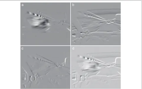
. Thus, the temporal gra-dient of an image requires at least five consecutive images of the sequence. The results of these convolutions are the estimates of the partial derivatives, which are shown in Figure 2, and represent the temporal, Figure 2a, hori-zontal, Figure 2b, vertical, Figure 2c, and global intensity changes, Figure 2d.
Finally, the velocity vectors associated to each pixel of the image are computed from the spatiotemporal partial derivatives previously computed. This is done by using a spatial neighborhood matrix of 5 ×5 pixels, centered
Figure 2Partial derivatives of an image in three dimensions:t,xandy.(a)Derivative int.(b)Derivative inx.(c)Derivative iny.(d)Derivatives int,x, andy.
on each pixel, and a one-dimensional weight matrix, (0.0625, 0.25, 0.375, 0.25, 0.0625), [24]. The noise parame-ters used areσ1=0.08,σ2= 1.0, andσp =2.0 [57]. The
estimated velocity vectors whose highest eigenvalue of
ATW2Ais less than 0.05 are considered unreliable (noise) and are discarded [24].
3.2 Results of the sequential algorithm
Figure 3 shows the optical flow computed for the image of Figure 1a. The processing steps have been analyzed and are shown in Figures 1 and 2. The original image cor-responds to a three-lane highway. The vehicle carrying the camera is overtaking the vehicle on the right while it is being overtaken (quite fast) by the vehicle on the left. This introduces some noise in the results, since it would require a higher temporal resolution to correctly handle the movement of objects at such speed.
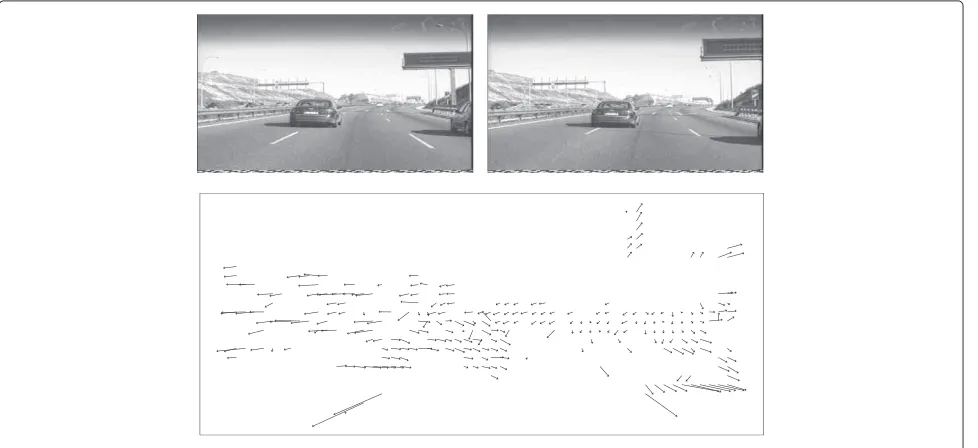
Figure 4 shows two images of a video sequence that has been processed with this algorithm and also the opti-cal flow obtained after applying this algorithm. In this sequence, a vehicle can be observed on the right going slower than the vehicle where the camera is installed, and a second vehicle on the left is changing lanes. Finally, a traffic light panel can be seen above. The optical flow generated by these three objects and by the road
lines and other elements on the shoulder are shown in Figure 4.
4 Sequential algorithm tasks and dependencies
This section analyzes in some detail the dependencies among the tasks of the sequential algorithm described in Section 3.1. The pseudocode of the algorithm’s main loop is shown below, including the task list with the task parameters.
/* Sequential algorithm main loop */
while (readfile (fname, time, raw_pic, ...)> 0) { T_Smooth (raw_pic, s_T_buff, ...);
X_Smooth (s_T_buff, s_TX_buff, ...); Y_Smooth (s_TX_buff, s_TXY_buff, ...); t_derivate (s_TXY_buff, diff_buff.It, ...); x_derivate (s_TXY_buff, diff_buff.Ix, ...); y_derivate (s_TXY_buff, diff_buff.Iy, ...);
velocities (diff_buff.Ix, diff_buff.Iy, diff_buff.It, vels_pic, ...); out_velocities (full_name, "Full", vels_pic, ...);
}
The tasks mentioned in the algorithm’s main loop are as follows:
• read_filereads images from disk and passes them to T_smooth.
• T_smoothreceives images fromread_fileand passes them to
X_smooth. Performs the temporal smoothing, using the current image as well as then previous images andn following images, withn=4·σ. This calculation involvesa very strong dependence between each image and all those around it. In fact, every image depends on another8·σimages. With a value ofσ=3.2that means the 12 previous and the 12 following frames.
• X_smoothreceives images fromT_smoothand passes them toY_smooth.Performs the spatial smoothing of the images on thexcoordinate. • Y_smoothreceives images fromX_smoothand
passes them tot_derivative,x_derivative, and
y_derivative. Performs the spatial smoothing of the images on theycoordinate.
• t_derivativereceives images fromY_smooth, calculates the partial derivative of the images with respect tot(It), and passes it tovelocities. Five images are required, two previous and two following the current one. This calculation is affected bya very strong dependency of each image with the four images surrounding it.
• x_derivativereceives images fromY_smooth, calculates the partial derivative of the images with respect tox(Ix), and passes it tovelocities. • y_derivativereceives images fromY_smooth,
calculates the partial derivative of the images with respect toy(Iy), and passes it tovelocities. • velocitiesreceives the partial derivatives with respect
tot,x, andyof the images (It,Ix, andIy) from t_derivative,x_derivative, and
y_derivative. Using these partial derivatives, it calculates each pixel velocity as a pair(vx,vy)and passes it toout_velocities.
• out_velocitiesreceives velocity vectors from velocitiesand processes them to generate the appropriate output. For example, it calculates statistics (splitflow) or converts them to
PostScript (psflow) to visualize the results. Finally, it writes the calculated speeds to disk.
Reviewing the major tasks that make up the application reveals a problem: the execution of the tasks must fol-low a strict order. Therefore, the parallel execution of the tasks inside a single iteration is not possible because their order must be respected. However, it is possible to over-lap the execution of tasks over different images. Moreover, there are strong dependencies between the input data, as T_smoothandt_derivativesneed to know not only the image being processed but also the neighbouring ones. Therefore, the optical flow from different images can-not be calculated in parallel without processing the other images.
5 Parallel algorithm
In order to parallelize the Lucas-Kanade algorithm, the dependencies described in Section 4 were the starting point to build a hybrid scheme. Data and computation have been parallelized by dividing the input image into subimages and distributing the tasks to be performed on each pixel. This form of combined algorithm is much more flexible than using parallelization on data or on tasks separately.
If only data parallelization were considered by dividing the images and executing the algorithm on every data sub-set on a medium-sized cluster (64 or more processors), very small images have to be considered. Even if large images are taken into account (2,000×1,200 pixels), the size of the subimages (250 × 150) is too small. On the other hand, to obtain correct results, pixel dependencies have to be considered for smoothing on all three coordi-nates and also when calculating the derivatives. Solving these dependencies requires introducing additional pixels, usually known as border pixels. If many subpictures are used, the number of border pixels (ghost or halo pixels) increases and the overhead costs of this algorithm would become unacceptable.
If only the tasks parallelization analyzed in Section 4 is considered, the task number is too low, even when the larger tasks are distributed between several nodes for load balancing. Initially, there are seven starting tasks, not including I/O. Even if some of those tasks are dou-bled or tripled, the execution does not benefit from a cluster with more than 14 to 16 processors. Furthermore,
in this scheme, dependencies do not have to be taken into account between pixels but between tasks.T_smooth and t_derivative tasks require knowing all of the images because previous and further images are needed when performing these computations. The best way to solve these dependencies is by using a pipeline. Images have to progress through the pipeline stages. To balance the duration of different stages, the longer stages have to be replicated. This solution solves one of the prob-lems, dependencies between tasks, but not the scalability problem.
If both solutions are combined, establishing a task pipeline and partitioning input images, an easily scalable and flexible scheme is obtained. The idea is to have a full pipeline for each subimage, i.e., several pipelines of N stages, with some of these replicated. The algorithm dependencies are solved and the border overhead is mini-mized because images are divided into a small number of subimages. Adding the border pixels allows treating each subimage independently. Smoothing on the X and Y coor-dinates uses 25 pixels, 12 on each side of the central pixel, hence, each subimage needs 12 more pixels. Therefore, to divide 1,280×1,024 images into four subimages (2×2), four 652×524 subimages are necessary, by adding 12 pix-els on theXandYaxis. In this way, the border pixels are overlapped, and every subimage is completely indepen-dent of others.
If the number of processors available is small, the use of a single pipeline is sufficient. If the number of proces-sors is lower than the number of pipeline stages, several tasks can be grouped to balance the load of the stages. This analysis will be addressed in Subsection 6.1.
If there are many processors available, several pipelines have to be built so that all processors can work in paral-lel. The number of pipelines is calculated by dividing the number of available processors by the number of pipeline stages.
Section 6 shows how the pipeline could be increased up to 16 stages. If every image is divided into 64 subim-ages, 1,024 processors can be used due to the scalability of this model. Obviously, using 1,024 processors would make sense for working with a high number of large images (large sequences or very high temporal resolu-tion). In most cases, a 16 to 64 processor cluster will be enough to process the input sequences in a reasonable time.
6 Pipeline structure
As shown in Section 5, a pipeline structure is proposed as the main idea to exploit parallelism. The optical flow application is divided into independent modules to be connected in the same sequential order of the tasks to be executed for each single image. When a module fin-ishes its processing task for an image, it starts execut-ing the same task for the next image. This way, each module is working on a different image at a certain time.
The objective of this structure is to create a thread for each of the tasks shown in Section 4. This way, a dif-ferent thread is assigned to each task and will execute its function on each of the images, in parallel with other threads that will be executing their function on different images.
The derivatives computation is not too demanding. However, the three tasks that solve the derivatives are grouped in order to simplify communication because the three tasks get the same input information from Y_smoothand send the results tovelocities. Conse-quently, the mapping task-thread is as follows:
• in_thexecutes the taskread_file. • smoothT_thexecutes the taskT_smooth. • smoothX_thexecutes the taskX_smooth.
• smoothY_thexecutes the taskY_smooth. • diff_thexecutes the taskderivativesthat
includes the derivative computation int,x, andy. • vels_thexecutes the taskvelocities.
• out_thexecutes the taskout_velocitiesthat includes thepsflow,splitflow, and writes results to the disk.
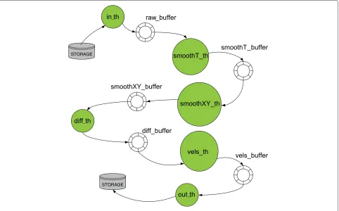
Because the time taken for each stage is different, sev-eral synchronizations will be introduced in the pipeline. As usual, buffers with synchronization mechanisms have to be introduced between threads to allow commu-nication between them. Figure 5 shows threads and buffers used for communication in the shared memory pipeline.
In order to measure the time spent on each task, a sequential implementation has been run on a single clus-ter node. Two image sizes have been used as input data:
720 × 576 and 502 × 288 pixels. The most important
result is the relationship between the times spent by different tasks, but not the time each task spends indi-vidually. Table 1 shows the amount of time spent on each task and its weight on the total time spent by the algorithm.
An important aspect to be pointed out is that the exe-cution time ratio for the tasks is constant even when
_
_ STORAGE
STORAGE _
Table 1 Execution time per task (ms)
Task Time 502×288 Time 720×576
read_file 0.9 ms 0.1% 0.9 ms 0%
T_smooth 12 ms 6.9% 40 ms 7.6%
X_smooth 8 ms 4.6% 30 ms 5.7%
Y_smooth 7 ms 4.1% 25 ms 4.8%
t_derivative 7 ms 4.1% 25 ms 4.8%
xy_derivatives 3 ms 1.7% 10 ms 1.9%
velocities 130 ms 74.4% 370 ms 70.4%
out_velocities 7 ms 4.1% 25 ms 4.8%
changing the image size. This fact allows using the same approach when parallelization is addressed, without tak-ing into account the image size.
Another aspect to be considered is that the temporal smooth is slower than the spatial smooth tasks. This is because spatial smooth works with just a single image, while temporal smooth requires several images preceding and following the one being processed. The main
differ-ence between the smooth on theX axis and the smooth
on theY axis is that the image can be in cache memory when the latter is executed. In the same way that tempo-ral smooth is slower than spatial smooth, the computation of the temporal derivative is slower than the computation of spatial derivatives. The reason is again the need of the temporal derivative to use several images, clearly spoiling the memory hierarchy behavior.
6.1 Pipeline stages
Table 1 shows that the execution times for different tasks are not well balanced, and this situation has to be changed. Taking into account the time spent on each task, a new organization of tasks is proposed. The main reason sup-porting the redesign of the pipeline stages is the high
exe-cution time for thevelocitiesfunction. The proposed
solution is to parallelize the slower task (velocities) since it does not depend on other images, but on the derivatives with respect tot,x, andy, i.e.,It,Ix, andIy. With the purpose of obtaining a higher speedup, the pipeline has initially been proposed for 16 processors, even if there are fewer processors. The scheme is valid as it is flexible enough to allow grouping tasks to adapt to
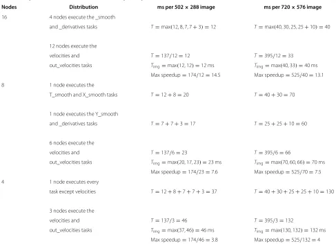
Table 2 Pipeline times (ms) and theoretical speedups
Nodes Distribution ms per 502×288 image ms per 720×576 image
16 4 nodes execute the _smooth
and _derivatives tasks T=max(12, 8, 7, 7+3)=12 T=max(40, 30, 25, 25+10)=40
12 nodes execute the
velocities and T=137/12=12 T=395/12=33
out_velocities tasks Timg=max(12, 12)=12 ms Timg=max(40, 33)=40 ms Max speedup=174/12=14.5 Max speedup=525/40=13.1
8 1 node executes the
T_smooth and X_smooth tasks T=12+8=20 T=40+30=70
1 node executes the Y_smooth
and _derivatives tasks T=7+7+3=17 T=25+25+10=60
6 nodes execute the
velocities and T=137/6=23 T=395/6=66
out_velocities tasks Timg=max(20, 17, 23)=23 ms Timg=max(70, 60, 66)=70 ms Max speedup=174/23=7.6 Max speedup=525/70=7.5
4 1 node executes every
task except velocities T=12+8+7+7+3=37 T=40+30+25+25+10=130
3 nodes execute the
velocities and T=137/3=46 T=395/3=132
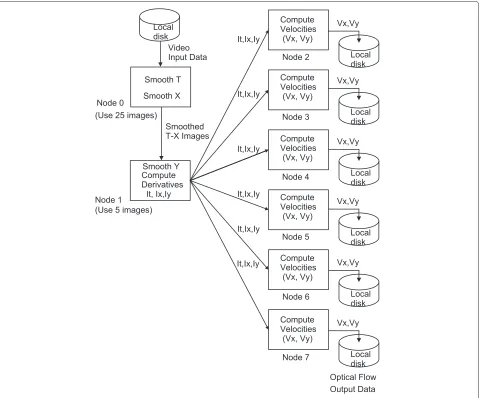
Figure 6Parallel algorithm structure for eight single processor nodes.
other situations. Table 2 shows how the task distribution is scheduled in the pipeline for 4, 8, and 16 nodes and the pipeline time per image for every case. Figure 6 details the task scheduling for each node when using an 8-node computer.
If a distributed memory computer is used, the commu-nication time has to be taken into account and will depend on the network used (Gigabit, Myrinet,...). However, this time is not negligible and tends to be around several milliseconds. This approach is also valid for a shared memory multiprocessor, minimizing the communication overhead.
7 Shared memory version with hyperthreading
The first implementation described used a shared mem-ory biprocessor with hyperthreading (i.e., four virtual
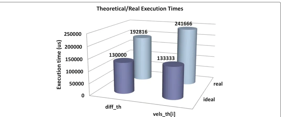
Figure 8Comparison between the theoretical and the actual execution times when using a computer with hyperthreading.
processors). Taking into consideration the parallel algo-rithm proposed in Section 6.1 for four processors, the following grouping of tasks has been made:
• diff_thperforms the tasksread_file,T_smooth, X_smooth,
Y_smoothandderivatives.
• vels_thperforms tasksvelocitiesand out_velocities.
As thevels_thtakes three times as long asdiff_th,
the idea is to execute three vels_th threads so that
the delay is compensated. Furthermore, this structure
can be carried out because tasks velocities and
out_velocities do not depend on other images,
instead, they only depend on the partial derivatives of a single image,It,Ix, andIy. In this way, execution times are better balanced and there is a better fit to the archi-tecture used with four threads running in four virtual processors. The communication scheme between threads is shown in Figure 7.
When measuring the execution times, it can be observed that the behavior of the threads is greatly influenced by the hyperthreading technology of the processors. Figure 8 shows the differences between the execution times theoretically calculated in Section 6 and the actual execution times measured when executing the application.
In Figure 8, it can be seen that actual execution times are much longer than theoretical times. Moreover, it
can be seen that threads vels_th suffer higher delays
(81% slower) than diff_th threads (48% slower). This
is because these threads, being all clones, compete for
the same functional units of virtual processors, producing conflicts and delays.
8 Message-passing version
The second implementation of the parallelized Lucas-Kanade algorithm is based on distributed memory with message-passing communications. This version has been developed and implemented on an eight-node cluster.
The tasks mentioned in Table 1 have been assigned to the eight nodes of the cluster, and the MPI message-passing standard has been used for communications.
To optimize the communications between nodes, asyn-chronous non-blocking messages have been used so that communications and computing are overlapped. Conse-quently, while a node is processing imagei, it has already started a non-blocking send with the results of process-ing the previous image (i-1), and it has also started a non-blocking reception to simultaneously receive the next image to be processed (i+1). In this way, simultaneous submissions, receptions, and computing are allowed in each node.
Moreover, persistent messages have been used to avoid building and destroying the data structures used for each message. This design decision has been possible because the information traveling between two given nodes always has the same structure and the same size so that the skeleton of the message can be reused.
The general communication scheme between different nodes is shown in Figure 6.
The scheme employed for the distribution of tasks over nodes was as follows:
/* Node-0 code. Use persistent messages and asynchronous communications */ ...
while (n_bytes = readfile (fname, raw_pic, ...)){
MPI_Wait(&request[comp], &status); /* Wait for the oldest send to finish */
T_smooth(raw_pic, s_T_buff[comp], ...);
X_smooth(s_T_buff[comp], s_TX_buff[comp], ...);
comp = (comp + 1) % N_SMOOTH_T_BUFFERS; out = (out + 1) % N_SMOOTH_T_BUFFERS;
MPI_ISend(&request[out]); /* Start the next asynchronous sending op. */ }
Node-0 code performs the following tasks: it reads the images of the video sequence from the disk, then it performs the temporal smoothing (using the current image as well as the previous 12 and the next 12 images) and performs the spatial smoothing on thexcoordinate. Finally, it sends the image smoothed ontand onxto node 1.
• Node 1: The pseudocode representing the job completed at node 1 follows
Node-1 performs the following tasks: it receives the images already smoothed ontandx, from node 0, then it performs the spatial smoothing on they coordinate, and computes the partial derivative with respect totof the image (using five images, the current one, plus the previous two and the next two). Finally, it sends the processed image to the other nodes, from 2 to 7, selecting the target in a cyclical way. • Rest of the nodes: The pseudocode that describes
the work done at the rest of the nodes follows
/* Node-0 code. Start an asynchronous receiving operation */ MPI_IRecv(&request_in[in]);
/* Start send/recv operations to overlap communication & computation */ ...
while (working) {
in = (in + 1) % N_SMOOTH_Y_BUFFERS;
MPI_IRecv(&request_in[in]); /* Start the next asynchronous receiving operation */
MPI_Wait(&request_in[comp_in], &status); /* Wait for the previous receive to finish*/
if ((status.MPI_TAG == END) || (status.MPI_ERROR != 0)) end();
MPI_Wait(&request_out[dest][comp_out], &status); /* Wait for the oldest send */
Y_smooth(X_s_buff[comp_in], Y_s_buff[comp_in], ...);
t_derivatives(s_Y_buff[comp_in], buff[dest][comp_out].It, ...);
MPI_ISend(&request_out[dest][comp_out]); /* Start the next asynchronous sending operation*/
comp_in = (comp_in + 1) % N_SMOOTH_Y_BUFFERS; if (++dest == nprocs) {
dest = FIRST_PROC_VELS;
comp_out = (comp_out + 1) % N_DIFF_BUFFERS; out = (out + 1) % N_DIFF_BUFFERS;
/* Rest of the nodes. Start an asynchronous receiving operation */ MPI_IRecv(&buff[comp], ...);
while (working) {
in = (in + 1) % N_DIFF_BUFFERS;
MPI_IRecv(&request_in[in]); /* Start the next asynchronous receiving operation */
MPI_Wait(&request_in[comp], &status); /* Wait for the previous receive to finish*/
if ((status.MPI_TAG == END) || (status.MPI_ERROR != 0)) end();
x_derivative (buff[comp].s_TXY, Ix, ...); y_derivative (buff[comp].s_TXY, Iy, ...);
velocities (Ix, Iy, buff[comp].It, vels_pic, ...); out_velocities(full_name, vels_pic, ...);
comp = (comp + 1) % N_DIFF_BUFFERS; }
Each node from 2 to 7 performs the following tasks: it receives images already smoothed int,x, andy, as well as the derivative with respect tot(It) of the image from node 1, then it calculates the partial derivatives with respect toxandyof the image, (Ix andIy). Starting from the derivatives int,x, andy (It,Ix, andIy) of the image, it computes the speed of each pixel as a pair(vx,vy)and formats the computed
velocities (statistics, etc.) before writing them to disk.
Taskxy_derivativeshas been taken from the inter-mediate node to the end nodes to reduce the size of the messages. Instead of sending three matrices per image (It,Ix, andIy), two matrices are sent, (Itand the image smoothed ont,x, andy). The task loads are not so well balanced but, by reducing the network traffic, the perfor-mance improves due to the communication time being shorter.
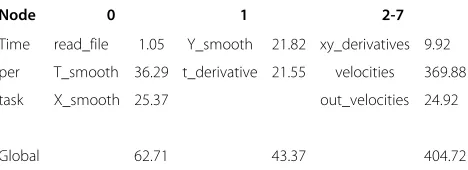
Table 3 shows the mean values for the time spent on each task and the global computing time spent by each node with every image.
From the data shown at Table 3, it can be observed that regardless of the waiting time spent on communication calls, the load is fairly well balanced between nodes 0 and 2 to 7. Node 1 is out of balance, as envisaged in the previous
Table 3 Mean time per task (ms)
Node 0 1 2-7
Time read_file 1.05 Y_smooth 21.82 xy_derivatives 9.92 per T_smooth 36.29 t_derivative 21.55 velocities 369.88
task X_smooth 25.37 out_velocities 24.92
Global 62.71 43.37 404.72
paragraph, and in actual terms the imbalance is even higher as will be shown. The theoretical estimates were made from the times obtained by executing the sequential version, which executes everything within the same node (and the same processor). Processing multiple images in the sequential version implies a heavy use of memory that can sometimes produce a high rate of page replacements, and even thrashing. The use of memory is not so heavy in the message-passing version, since the number of images handled by each node is much smaller.
9 Message-passing and threads
This section looks at a third implementation, imple-mented with 16 processors. The idea is based on maxi-mizing the use of resources available in the machine. As already mentioned, a cluster of eight dual processors with hyperthreading nodes is used. However, due to the bad results obtained with hyperthreading shown in Section 7, only the real processors have been used instead of the virtual ones.
This implementation is based on threads and MPI. The goal is to run several threads in each node, thereby taking advantage of the existence of two processors on every sin-gle node. The threads in the different nodes communicate using MPI.
Due to the single-threaded MPI implementation used, it is only possible to make invocations to the MPI library from a single thread. Thus, a single thread responsible for communications has been assigned to each node to send and receive messages, and it is the only one interacting with the MPI library. This thread is normally suspended and only wakes up when data to send or receive are available.
are persistent to reuse their skeleton, as in the implemen-tation described in Section 8.
A sending window has been implemented in order to maximize the overlapping of data communication and computation. A variable pointing to the next element to be sent and a variable pointing to the next message to be confirmed by node are maintained. The communication buffers are circular allowing the same memory locations to be reused for different images along the execution of the program.
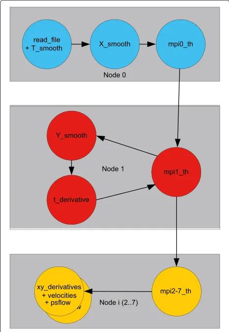
The division of tasks is based on the algorithm for 16 processors described in Subsection 6.1. In any case, the distribution of tasks to nodes is the same as in the previ-ous version, shown in Figure 6. The differences are found inside each node as described in the following subsections, since multiple threads run in each node as shown in Figure 9.
9.1 Node 0
Three of the tasks described in Section 6 run on node 0. The first two,read_fileandT_smooth, are grouped in
Figure 9Parallel algorithm structure using eight dual processor nodes, with MPI and threads.
a single thread, since the former takes a very short time, andX_smooth runs on another thread. A third thread, mpi0_th, is responsible for communication of this node with the next one (node 1).
9.2 Node 1
Two of the tasks described in Section 6 run on node 1.
One thread executes the task Y_smooth and an other
thread executes the taskt_derivative. A third thread, mpi1_th, is responsible for communication of this node with node 0 and with nodes 2 to 7.
9.3 Nodes 2 to 7
Three of the tasks described in Section 6 run on each of the nodes 2 to 7. An important difference from the other nodes is the absence of dependencies between images within these tasks. Consequently, a single thread can han-dle all three tasks for a given image, reusing the data in memory.
Specifically, there will be one thread per proces-sor (velocities_th[0-1]). Each is responsible
for the computation of the derivatives in X and Y
(xy_derivatives), the computation of the velocity vec-tors (velocities), the formatting of the output (using psflowandsplitflow), and dumping the output to disk (out_velocities). An additional thread, mpi2-7_th, will handle communications with node 1.
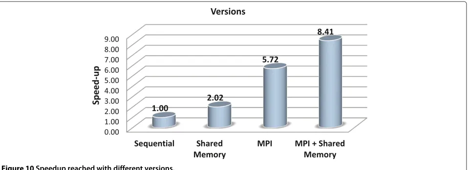
10 Results
Figure 10 shows the speedup reached by different ver-sions. This section analyzes the results for each version implemented.
10.1 Cluster architecture
Parallelization has been carried out in a generic way in order to be sufficiently general to serve for different archi-tectures, either based on distributed or on shared mem-ory. Performance measures have been obtained using an architecture based on distributed multiprocessor nodes so that the evaluation of the different implementations has been possible.
Figure 10Speedup reached with different versions.
components are replicated while others must be shared between processes or threads.
10.2 Shared memory version
With the shared memory version, a speedup of 2.02 was obtained, i.e., it runs twice as fast as the sequential ver-sion. Without taking into account the type of operations performed by the application and the details of the pro-cessors, a higher improvement would be expected.
A first reason to explain the relatively low speedup is the amount of memory needed by the application. The sequential version needs a much lower amount of mem-ory than the threads version, and memmem-ory accesses are performed in a more sequential way so that processing of an image finishes before moving on to the next one. In the case of shared memory, several images are han-dled simultaneously, each one corresponding to a different processing time. It also needs to access scattered memory positions, so it requires a larger memory and uses it in a less efficient way because of the irregular memory access pattern.
Another cause for the low speedup is the use of hyper-threading technology. While every node apparently has four processors (dual-hyperthreading processor), there are just two actual processors. Analyzing the application code, it can be noted that the calculations basically con-sist of floating point operations (floating point square roots, multiplications, etc.). Considering the usual struc-ture of current processors, it is clear that the floating point functional units are not sufficiently replicated.
In an attempt to distinguish inefficiencies due to the par-allel implementation - such those due to distribution of tasks - from speed-up limitations due to the supporting architecture, a common, highly parallelizable application example has been used as a reference. The example is the matrix multiplication and the speedup reached in this case is 2.7, far from the theoretical maximum 4. From
this result, the application speedup obtained, 2.02, can be considered as reasonable.
10.3 Message-passing version
Sending a message from one node to another may be very time-consuming, depending on the network charac-teristics and the amount of information being transferred. However, communication between nodes is asynchronous so, at least in part, it may be possible to overlap com-munication operations (both sending and receiving) with CPU processing time. Due to the non-blocking charac-teristics of the application communications, the program does not need to wait for sending or receiving operations to finish, but instead it immediately begins to perform the calculation on the data already available.
With this communication scheme based on non-blocking and persistent messages, a higher speedup than the one shown in Figure 10 could be expected. The analy-sis of the execution time of all tasks, both in the sequential and in the message-passing versions, shows that the time spent was very similar, which points to communications as the origin of the performance problem. Lower than expected performance of the message-passing implemen-tation is mainly due to the large volume of data exchanged. There are two types of messages: those exchanged between nodes 0 and 1 and the messages that node 1 sends to the end nodes (2 to 7). Node 0 sends data after applying a smooth function to the image on coordinates
T andX. The amount of data sent for each image is then equivalent to a floating point number per image pixel. The image resolution used for experimentation is 720 ×576 pixels, so the total data sent per image are 720·576 = 414, 720 float elements, or 414, 720 float·4(bytes/float)= 1, 658, 880 B.
Mbps, the delivery time per message sent from node 0 to node 1 would be
1, 658, 880 B·8(bits/byte)/800 Mbps=16.58 ms.
As for the size of the message sent by node 1 to pro-vide end nodes with the data they need, it must be noted that it is sent after t derivatives are computed (It). In fact, not only such derivatives but also smoothed images have to be sent to allow computingxandyderivatives. Therefore, two matrices as large as the matrix sent from node 0 to node 1 have to be sent, needing twice as much time.
Summarizing, the large amount of data transferred explains why the performance achieved is lower than the theoretical maximum.
Anyway, with this parallelization scheme, the computa-tion of the optical flow achieves a throughput of 30 images per second with 502×288 pixel images. For 720×576 pixel images, the throughput obtained is ten images per second.
10.4 Message-passing and shared memory version
The last version considered tries to take advantage of the previous two. This combined version parallelizes at node-level using threads and at the network node-level by making use of MPI.
Comparing this version with the message-passing one, it must be noted that the task distribution among nodes is the same in both versions. It was considered important to compare both versions in order to analyze the benefit of introducing shared memory mechanisms. In this case, the number of threads created, as well as their features, makes it easier to appreciate the performance reachable with this technique. In comparison with the message-passing ver-sion, the speedup of the final version is 1.47, which is quite significant.
With this version, the computation of the optical flow achieves a throughput of 45 images per second with 502× 288 pixel images. For the 720×576 resolution, 15 images per second throughput is obtained. Note that in both cases the optical flow is computed for every image.
11 Conclusion
This paper addresses the parallelization of optical flow calculation. A flexible and scalable parallelization scheme has been described, based on dividing each image into several subimages in order to process each one through a software pipeline. This pipeline allows to respect dependencies between different computation stages. Each pipeline step performs an optical flow computation stage. Stages exhibiting a greater need for computation are repli-cated to balance the time spent on each pipeline stage. The number of subimages which each image is divided into depends on the number of processors available, thus ensuring high scalability. This parallelization scheme has
been developed starting from a dependency analysis of the Lucas-Kanade algorithm, using a sequential implementa-tion developed at the University of Porto.
Three different versions of the proposed scheme have been implemented and executed on a cluster of dual hyperthreading processor nodes to evaluate its flexibility and scalability. These versions are as follows:
• A shared memory version, using threads. It yields a speedup of 2.02 on a four-processor system. • A distributed memory version using MPI. In an
eight-processor system it yields a speedup of 5.72. • A hybrid version, using threads and MPI to take
advantage of the fact that each node is a
multiprocessor - a dual hyperthreading processor. In an eight-node system, with two processors per node, the speedup reached is 8.41.
The speedup obtained in all three cases is very satis-factory, clearly showing the feasibility of the proposed scheme, as well as its flexibility and scalability. If more than 16 processors are going to be used, this task pipeline can be combined with image partitioning, having a full pipeline consisting of 16 stages per subimage.
Once implemented, these versions have been used to calculate optical flow video sequences taken in variable natural-light conditions and with a moving camera. In fact, the camera was installed on board a vehicle travel-ing on conventional open roads. Despite the challengtravel-ing conditions of these experiments, the results obtained were satisfactory.
This parallelization scheme can be combined with GPUs. Each task of the pipeline can be implemented as a kernel in a GPU to improve the performance, as current GPUs are very powerful and affordable. As three different versions of the task pipeline have been proposed, with 4, 8, or 16 processors, the solution can be easily adapted to a different number of GPUs to take advantage of a GPU cluster.
The use of these kinds of coprocessors, MICs or GPUs, can improve drastically the performance of the paralleliza-tion scheme described in this paper.
Competing interests
The authors declare that they have no competing interests.
Received: 22 July 2013 Accepted: 13 February 2014 Published: 28 March 2014
References
1. SS eauchemin, JL Barron, The computation of optical flow. ACM Comput. Surv.27(3), 433–466 (1995)
2. X Feng, P Perona, Scene segmentation from 3D motion, inIEEE Computer
Society Conference on Computer Vision and Pattern Recognition,Santa
Barbara, 23–25 June 1998 (IEEE Computer Society Los Alamitos, 1998), pp. 225–231
3. S Temizer,Optical flow based local navigation. (PhD thesis, Massachusetts Institute of Technology, Cambridge, MA, 2001)
4. JS Zelek, Towards Bayesian real-time optical flow.Image Vis. Comput. 22(12), 1051–1069 (2004)
5. Z Wei, DJ Lee, BE Nelson, KD Lillywhite, Accurate optical flow sensor for obstacle avoidance, inProceedings of the 4th International Symposium on
Advances in Visual Computing,Las Vegas, 1–3 December 2008, LNCS,
vol. 5358 (Springer Berlin, 2008), pp. 240–247
6. J Marzat, Y Dumortier, A Ducrot, Real-time dense and accurate parallel optical flow using CUDA, in17th International Conference WSCG,Plzen, 2–5 February 2009, pp. 105–111
7. P Sand, SJ Teller, Video matching. ACM Trans, Graph.23(3), 592–599 (2004) 8. F Champagnat, A Plyer, G Le Besnerais, B Leclaire, B Davoust, Y Le Sant,
Fast and accurate PIV computation using highly parallel iterative correlation maximization. Exp. Fluids.50(4), 1169–1182 (2011) 9. F Valentinotti, GD Caro, B Crespi, Real-time parallel computation of
disparity and optical flow using phase difference. Mach Vis. Appl. 9(3), 87–96 (1996)
10. F Weber, H Eichner, H Cuntz, A Borst, Eigenanalysis of a neural network for optic flow processing. New J. Phys.10(1), 015013 (2008)
11. K Sakurai, S Kyo, Okazaki S, Overtaking vehicle detection method and its implementation using IMAPCAR highly parallel image processor. IEICE Trans.91-D(7), 1899–1905 (2008)
12. T Röwekamp, M Platzner, L Peters, Specialized architectures for optical flow computation: a performance comparison of ASIC, DSP, and multi-DSP, inProceedings of the 8th ICSPAT,San Diego, 14–17 September 1997, pp. 829–833
13. J Kramer, Compact integrated motion sensor with three-pixel interaction. IEEE Trans. Pattern Anal. Mach. Intell.18(4), 455–460 (1996)
14. M Fleury, AF Clark, AC Downton, Evaluating optical-flow algorithms on a parallel machine. Image Vis. Comput.19(3), 131–143 (2001)
15. JH Barrón-Zambrano, FM del Campo-Ramírez, M Arias-Estrada, Parallel processor for 3D recovery from optical flow, inInternational Conference on
Reconfigurable Computing and FPGAs,Cancun, 3–5 December 2008 (IEEE
Computer Society Los Alamitos, 2008), pp. 49–54
16. S Tan, J Dale, A Anderson, A Johnston, Inverse perspective mapping and optic flow: a calibration method and a quantitative analysis. Image Vis. Comput.24(2), 153–165 (2006)
17. K Sakurai, S Kyo, S Okazaki, Overtaking vehicle detection method and its implementation using IMAPCAR highly parallel image processor. IEICE Trans.91-D(7), 1899–1905 (2008)
18. C Braillon, C Pradalier, J Crowley, C Laugier, Real-time moving obstacle detection using optical flow models, in2006 IEEE Intelligent Vehicles
Symposium,Tokyo, 13–15 June 2006, pp. 466–471
19. K Pauwels, MM Van Hulle, Optic flow from unstable sequences through local velocity constancy maximization. Image Vis. Comput.27(5), 579–587 (2009)
20. G Zhang, J Jia, HBao WHua, Robust bilayer segmentation and motion/depth estimation with a handheld camera. IEEE Trans. Pattern Anal. Mach. Intell.33(3), 603–617 (2011)
21. YS Hsieh, YC Su, LG Chen, Robust moving object tracking and trajectory prediction for visual navigation in dynamic environments, inIEEE
International Conference on Consumer Electronics (ICCE),Las Vegas, 13–16
June 2012, pp. 696–697
22. B Lucas, T Kanade, An iterative image registration technique with an application to stereo vision, inProceedings of the 7th International Joint
Conference on Artificial Intelligence (IJCAI),Vancouver, 24–28 August 1981,
pp. 674–679
23. B Lucas,Generalized image matching by method of differences. (PhD thesis, Department of Computer Science, Carnegie-Mellon University, 1984) 24. J Barron, D Fleet, SS Beauchemin, Performance of optical flow techniques.
Int. J. Comput. Vis.12(1), 43–47 (1994)
25. A Bainbridge-Smith, R Lane, Determining optical flow using a differential method. Image Vis. Comput.15(1), 11–22 (1997)
26. M Correia, A Campilho, J Santos, L Nunes, Optical flow techniques applied to the calibration of visual perception experiments, inProceedings of the
13th International Conference on Pattern Recognition, ICPR96,Vienna, 25–29
August 1996 vol.1, (1996), pp. 498–502
27. M Correia, A Campilho, Implementation of a real-time optical flow algorithm on a pipeline processor, inProceedings of the International Conference of Computer Based Experiments, Learning and Teaching,
Szklarska Poreba, 28 September to 1 October, (1999)
28. J Díaz, E Ros, R Agís, JL Bernier, Superpipelined high-performance optical-flow computation architecture. Comput. Vis. Image Underst. 112(3), 262–273 (2008)
29. T Brox, A Bruhn, N Papenberg, J Weickert, High accuracy optical flow estimation based on a theory for warping, inEuropean Conference on
Computer Vision (ECCV),Prague, 11–14 May 2009, LNCS,vol. 3024, ed. by
T Pajdla, J Matas (Springer Berlin, 2004), pp. 25–36
30. SN Tamgade, VR Bora, Motion vector estimation of video image by pyramidal implementation of Lucas Kanade optical flow, in2nd International Conference on Emerging Trends in Engineering and Technology
(ICETET),16–18 December 2009 (IEEE Computer Society Piscataway,
2009), pp. 914–917
31. A Doshi, AG Bors, Smoothing of optical flow using robustified diffusion kernels. Image Vis. Comput.28(12), 1575–1589 (2010)
32. A Bruhn, J Weickert, C Schnörr, Lucas/Kanade meets Horn/Schunck: combining local and global optic flow methods. Int. J. Comput. Vis. 61(3), 211–231 (2005)
33. M Drulea, IR Peter, S Nedevschi, Optical flow a combined local-global approach using L1 norm, inProceedings of the 2010 IEEE 6th International Conference on Intelligent Computer Communication and Processing, ICCP ’10,Cluj-Napoca, 26–28 August 2010 (IEEE Computer Society Piscataway, 2010), pp. 217–222
34. T Brox, J Malik, Large displacement optical flow: descriptor matching in variational motion estimation. IEEE Trans. Pattern Anal. Mach. Intell. 33(3), 500–513 (2011)
35. H Liu, TH Hong, M Herman, R Chellappa, Accuracy vs. efficiency trade-offs in optical flow algorithms, in4th European Conference on Computer Vision,
Cambridge, 15–18 April 1996, LNCS,vol. 1065, ed. by B Buxton, R Cipolla (Springer Berlin, 1996), pp. 271–286
36. B Buxton, B Stephenson, H Buxton, Parallel computations of optic flow in early image processing. Commun. Radar Signal Process. IEE Proc. F. 131(6), 593–602 (1984)
37. PE Danielsson, P Emanuelsson, K Chen, P Ingelhag, C Svensson, Single-chip high-speed computation of optical Flow, inMVA’90 IAPR Workshop on
Machine Vision Applications,Tokyo, 28–30 November 1990, pp. 331–336
38. G Adorni, S Cagnoni, M Mordonini, Cellular automata based optical flow computation for “just-in-time” applications, inInternational Conference on
Image Analysis and Processing,Venice, 27–29 September 1999,
pp. 612–617
39. A Stocker, R Douglas,Computation of Smooth Optical Flow in a Feedback
Connected Analog Network. (MIT Press, Cambridge, 1998).
http://cogprints.org/82/
40. H Bulthoff, J Little, T Poggio, A parallel algorithm for real-time computation of optical flow. Nature.337(6207), 549–553 (1989) 41. Del Bimbo A, P Nesi, Optical flow estimation on Connection-Machine 2, in
Proceedings of Computer Architectures for Machine Perception, New Orleans,
15–17 December 1993, pp. 267–274
42. H Wang, J Brady, I Page, A fast algorithm for computing optic flow and its implementation on a transputer array, inProceedings of the British Machine
43. C Colombo, A Del Bimbo, S Santini, A multilayer massively parallel architecture for optical flow computation, inProceedings of the 11th IAPR International Conference on Pattern Recognition, 1992. Vol. IV. Conference D:
Architectures for Vision and Pattern Recognition,The Hague, 30 August to 3
September 1992, pp. 209–213
44. MG Milanova, AC Campilho, MV Correia, Cellular neural networks for motion estimation, in15th International Conference on Pattern Recognition
(ICPR‘00),Barcelona, 3–7 September 2000 (IEEE Computer Society
Los Alamitos, 2000), pp. 819–822
45. H Niitsuma, T Maruyama, High speed computation of the optical flow, in
Proceedings of the 13th International Conference Image Analysis and
Processing - ICIAP 2005,Cagliari, 6–8 September 2005, LNCS,vol. 3617,
ed. by F Roli, S Vitulano (Springer Berlin, 2005), pp. 287–295 46. J Sosa, J Boluda, F Pardo, R Gómez-Fabela, Change-driven data flow
image processing architecture for optical flow computation. J. Real-Time Image Process.2(4), 259–270 (2007)
47. T Browne, J Condell, G Prasad, T McGinnity, An investigation into optical flow computation on FPGA hardware, inInternational Conference on
Machine Vision and Image Processing, 2008. IMVIP ’08,Portrush, 3–5,
September 2008, pp. 176–181
48. N Devi, V Nagarajan, FPGA based high performance optical flow computation using parallel architecture. Int. J. Soft Comput. Eng. 2(1), 433–437 (2012)
49. Y Mizukami, K Tadamura, Optical flow computation on compute unified device architecture, inProceedings of the 14th International Conference
Image Analysis and Processing - ICIAP 2007,Modena, 10–14 September
2007, pp. 179–184
50. M Gong, Real-time joint disparity and disparity flow estimation on programmable graphics hardware. Comput Vis. Image Underst. 113(1), 90–100 (2009)
51. MV Correia, AC Campilho, A pipelined real-time optical flow algorithm, in
Proceedings of Image Analysis and Recognition ICIAR (2),Porto, 29
September to 1 October 2004, LNCS,vol. 3212, ed. by AC Campilho, MS Kamel (Springer Berlin, 2004), pp. 372–380
52. J Chase, B Nelson, J Bodily, Z Wei, DJ Lee, Real-time optical flow calculations on FPGA and GPU architectures: a comparison study, in
16th International Symposium on Field Programmable Custom Computing
Machines,Palo Alto, 14–15 April 2008 (IEEE Los Alamitos, 2008),
pp. 173–182
53. (2014). http://www.top500.org Accessed 6 Mar 2014
54. A García Dopico, M Correia, J Santos, L Nunes, Distributed computation of optical flow, in4th International Conference on Computational Science
(ICCS 2004): 6-9 Jun 2004; Krakow, LNCS,vol. 3037, ed. by M Bubak,
G van A lbada, P Sloot, J Dongarra (Springer Berlin, 2004), pp. 380–387 55. T Kohlberger, C Schnorr, A Bruhn, J Weickert, Domain decomposition
for variational optical-flow computation. IEEE Trans. Image Process. 14(8), 1125–1137 (2005)
56. EM Kalmoun, H Köstler, U Rüde, 3D optical flow computation using a parallel variational multigrid scheme with application to cardiac C-arm CT motion. Image Vis. Comput.25(9), 1482–1494 (2007)
57. E Simoncelli, E Adelson, D Heeger, Probability distributions of optical flow,
inProceedings of the IEEE Conference on Computer Vision and Pattern
Recognition,Maui, 3–6 June 1991, pp. 310–315
doi:10.1186/1687-5281-2014-18
Cite this article as:Garcia-Dopicoet al.:Parallelization of the optical flow computation in sequences from moving cameras.EURASIP Journal on Image
and Video Processing20142014:18.
Submit your manuscript to a
journal and benefi t from:
7Convenient online submission
7 Rigorous peer review
7Immediate publication on acceptance
7 Open access: articles freely available online
7High visibility within the fi eld
7 Retaining the copyright to your article