Smart Align—a new tool for robust non-rigid registration of scanning microscope data

R E S E A R C H

Open Access

Smart Align

—

a new tool for robust non-rigid

registration of scanning microscope data

Lewys Jones

, Hao Yang

, Timothy J. Pennycook

, Matthew S. J. Marshall

, Sandra Van Aert

, Nigel D. Browning

,

Martin R. Castell

and Peter D. Nellist

Abstract

Many microscopic investigations of materials may benefit from the recording of multiple successive images. This can include techniques common to several types of microscopy such as frame averaging to improve signal-to-noise ratios (SNR) or time series to study dynamic processes or more specific applications. In the scanning transmission electron microscope, this might include focal series for optical sectioning or aberration measurement, beam damage studies or camera-length series to study the effects of strain; whilst in the scanning tunnelling microscope, this might include bias-voltage series to probe local electronic structure. Whatever the application, such investigations must begin with the careful alignment of these data stacks, an operation that is not always trivial. In addition, the presence of low-frequency scanning distortions can introduce intra-image shifts to the data. Here, we describe an improved automated method of performing non-rigid registration customised for the challenges unique to scanned microscope data specifically addressing the issues of low-SNR data, images containing a large proportion of crystalline material and/or local features of interest such as dislocations or edges. Careful attention has been paid to artefact testing of the non-rigid registration method used, and the importance of this registration for the quantitative interpretation of feature intensities and positions is evaluated.

Keywords:Image registration; Non-rigid registration; Quantitative ADF; Strain mapping; Principle component analysis; Scanning tunnelling microscopy (STM)

Background

Scanning microscopes are unique in that they allow for the recording of multiple signal types, often concur-rently, all of which are spatially resolved. For the study of material science, some of the most powerful families of instruments used are the aberration-corrected scan-ning transmission electron microscope (STEM), the scanning tunnelling microscope (STM) and atomic force microscope (AFM). Each of these valuable research tools is capable of yielding several imaging and spectroscopic signals, often in parallel, at atomic resolution. To re-trieve these spatially resolved signals, a scanned probe of either electrons or a physical tip is used, in contrast with the parallel illumination in conventional transmission electron (TEM) or optical microscopy. However, in each case, this serial acquisition comes with a penalty, as typ-ical acquisition times can be up to tens of seconds long

depending on the image dimensions and scanning speed. At these acquisition times, the operator has to worry about correcting not only image offsets from stage/sample drift [1–6] (for example from thermal expansion) but also low-frequency distortions that can perturb the image lo-cally [7–9]. Still, further problems can arise from incorrect instrument scan generator calibration [10]. These offsets and distortions then require correction by so-called rigid and non-rigid registrations.

Here, we present a new automated software for the robust non-rigid registration of serial microscopy data. First, in the Non-rigid registration section, non-rigid registration will be introduced along with some of the challenges specifically applicable to high-resolution mi-croscopy. Next, we describe the prior knowledge from the scanned nature of serial microscopy and how this can be used to design improved registration algorithms. In the Evaluation of the non-rigid performance section, the proposed methods are evaluated quantitatively with special interest paid to the frequency range of instabilities * Correspondence:[email protected]

1_{Department of Materials, University of Oxford, Oxford, UK}

Full list of author information is available at the end of the article

that can be corrected, the correction of small sample rota-tions and the robustness to registration artefacts. Lastly, in the Application to quantitative imaging section, some ap-plications of the new tool are presented, including: fidelity of quantitative annular dark-field (ADF) intensity and structural data as well as applications to scanning tunnel-ling microscopy (STM). Whilst not discussed here expli-citly, the methods developed are also applicable to other scanned microscopies such as atomic force microscopy.

Frequency purview of image registration methods

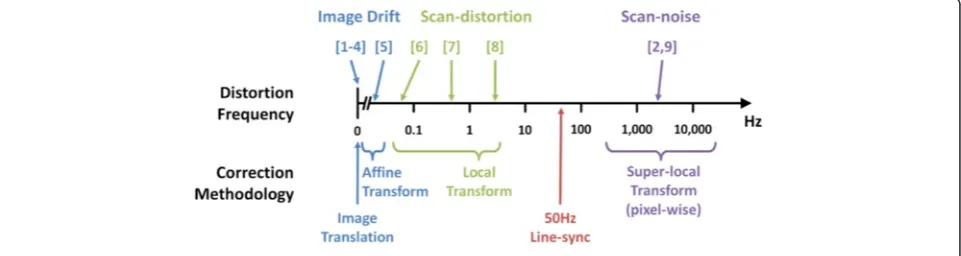
Before presenting our new algorithm, it is worth consider-ing the wider background of image registration regimes. Serial acquisition artefacts can be broadly grouped into low-, intermediate- and high-frequency issues and are often referred to as sample/image drift, scan distortion and scan noise, respectively. Various methods have been proposed to correct for these distortions, with the ap-proach tailored to the frequency range of the issue (Fig. 1). Rigid registration is the most simple of all the transfor-mations as one data is purely translated with respect to another; that is, all points in the data are shifted by the same vector. Many techniques have been proposed for this, using cross-correlation, mutual information [11] or Fourier space analysis [12, 13]. In this work, we will not comment on the well-established rigid registration (fur-ther background in [14]); instead, we will focus on dy-namic distortions and non-rigid registration.

Perhaps, the most commonly observed corruption of atomic resolution serial-acquired data is image drift. This is observable as a shearing of the known crystallo-graphic angles which becomes worse with slower scans (longer total frame time) or faster stage drift. One ap-proach to correcting this in STEM is to compare the ser-ial data with its conventional TEM counterpart. Using this, an affine transformation can be defined that cor-rects for the observed drift [1]. Whilst this is useful in that it can be performed on a single STEM image, this approach requires a mode change of the instrument making it challenging or impossible to work with the same region of interest. Another recent approach has

been to precess the instrument’s scan rotation, thus

varying the angle between the drift vector and the slow-scan direction (most sensitive to drift). This may be a comparison of two data recorded with perpendicular

scans [6–15], or with a sweep of many scan directions

[5] or even spiral scans [16]. In general, these measure-ments assume the drift rate remains constant although in [5], the authors demonstrated an adaptation to in-clude a slowly decaying drift rate. This adaptation then extends the scope of affine corrections from the ‘

zero-frequency’ of constant drift to the few tens of image

frames per cycle, say 0.005 Hz. To consider any image distortion frequency higher than this, affine transforma-tions can no longer be used and we must consider non-rigid registration.

Non-rigid registration

Non-rigid image registration refers to the transformation of imaging data from one coordinate set to another. Unlike simple affine transformations (translation, rota-tion, dilarota-tion, shearing etc.), non-rigid transformations do not necessarily preserve straight lines as different sub-regions of images may move by differing vectors. Such non-rigid registration has many applications in im-aging where either the object or recording process vary over time including remote sensing [17], medical im-aging [18, 19] and astronomy and photography [20]. In serial microscopy, the same challenges can be encoun-tered, with dynamic sample behaviour and instrumental instabilities both contributing to erroneous data offsets.

Non-rigid registration approaches in serial microscopy

Many approaches for non-rigid registration exist in other fields [14]; however, its use in microscopy is rela-tively recent, and few generalised methods exist. One ap-proach is to record experimental image series (time series) from which the effects of time-varying distortions and persistent sample information can be separated. These data can be reregistered by defining the so-called control points that appear in both data and determining a transformation operator to map these to each other.

Fig. 1Scanned image artefact types, frequency ranges and remedies

However, here, manual input is generally necessary in de-fining the control points which can be challenging and hampers automation. Instead, an alternative‘gradient

des-cent’ method, where the differences between images are

used to directly infer the direction of local motion [7–18], is well suited to automation and is what is discussed here.

In the gradient descent method, the differences be-tween the gradients of two grayscale images are used to suggest the displacement field between them. The

dis-placement map is applied to the ‘moving’ image. The

images are compared again and a new displacement field calculated (smaller than the first) which is added to the displacements already measured. In this way, the cumu-lative displacement needed to register the two images is built up iteratively. Estimating the displacement is an unconstrained problem and can lead to abrupt discon-tinuities in displacement and so requires a regulariser. In Berkels et al. [7], the Dirichlet energy of the displace-ment map is used as the regulariser in a variational ap-proach with a gradually reducing domain over which the Dirichlet energy is calculated. Importantly, and especially relevant to images of periodic structures such as atomic resolution micrographs, the transformation fieldmustbe smoothed sufficiently that no crystallographic features are seen in the diagnosed displacement field; if such periodicity is observable, then this represents an artefact of the diagnosis procedure itself and may compromise the final result. Here, we devise and apply a regularisa-tion approach specifically tailored for scanned images.

Non-rigid registration challenges

There are several effects that can impede the accurate registration of images including some challenges that are unique to atomic resolution micrographs. These can be sample related to the following:

Strong periodicity in the sample (crystallinity) Local structure variations that are genuine features

(not distortions) which must be preserved Structural changes in the sample due to sample

rotation, dynamic processes or damage effects [21,22], Changes in a STEM image’s constant background

from contamination etc. or in STM/AFM from tip-height changes.

or imaging related to the following:

Limited image signal-to-noise ratio (SNR)

A large constant background to the data (sometimes called‘black-level’or‘D.C. offset’)

Low-frequency (a few cycles per frame time) scan distortion

Changes in image appearance during STEM focal series from residual aberrations [23]

Changes in the image’s dynamic range or contrast during STEM focal [24] or camera-length series [25] or STM bias-voltage series [26]

Methods

The non-rigid method used in this work is based on the so-called gradient descent technique where the differences in the gradients of two image data are used to diagnose the position varying offsets between them. Specifically, the

accelerated ‘demons’ method [27] based on the work of

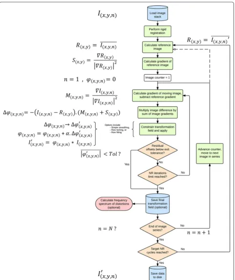
Cachier et al. [18] and Wang et al. [19] where more de-tailed background mathematics is described. Figure 2 shows an outline of the method used which will first be discussed before presenting experimental results.

Figure 2 shows the data setI(x,y,n)being imported from

disc, but in principle, the method can be modified to run in real time during data acquisition. Notation here is that images have lateral dimensions x-y and a counting index n. In the discussion presented here, the data are assumed to have already been rigid registered [11–13]. An initial reference image, R(x,y), is calculated by simply

taking the mean through the image series. The normal-isedxandygradient of this‘static’image,S, is calculated outside of the image series loop. Within the innermost iterative loop, the same normalised gradient is calcu-lated,M(x,y,n), this time for the moving (nth) image. The

difference between the intensity of the moving and static images, multiplied by the sum of the gradients, then yields the incremental transformation fieldΔφ(x,y,n).

Next, the incremental transformation field Δφ(x,y,n)

must be constrained in some way to yield a modified version of itself. The most simple modification would be smoothing to avoid discontinuities; tailoring the extent of this smoothing and more advanced treatments are discussed later. This yields the constrained incremental transformation field, Δφ’(x,y,n), which indicates the

non-rigid displacement field needed to bring the moving image towards registry with the reference. On the first loop of this innermost iteration, this represents the en-tire transformation measurement, φ(x,y); for subsequent

iterations, the incremental transformation field is multi-plied by a constantαadded to this.

Fig. 2Flow diagram of the non-rigid registration software algorithm. See the main text for a description of the symbols. Thedashed linerepresents an optional intra-loop update of the reference image

value ofαcan be optimised by evaluating the number of iterations to reach convergence ,but values between three and seven have been found to be reasonable in tests to date for images normalised in the dynamic range of zero-to-one and with approximately 20 pixels per atomic feature separation. If the solution converges very slowly, the user may increase the value of α, whereas if the offset diagnosis solution ‘bounces’, the value should be reduced.

Using the diagnosed transformation field, the experi-mental image is resampled over new grid points to affect this transformation and yield the intermediate image,I’n. Now, we have a new image, but this is only partly regis-tered, and soI’n, is analysed again iteratively to‘build up’ the full displacement diagnosis. Once complete, we move to the next experimental image in the series.

At the outset, we start with the assumption that the raw frames may be distorted, and so, it is also reasonable to assume that the reference image, the average over the frames, may be imperfect. As the low-frequency scan distortions are generally uncorrelated (random) between frames, then this blurring is sufficiently isotropic and unbiased. To achieve the best possible non-rigid results, the distortion-corrected frames of the first iteration are reused to create a new reference image and the process repeated. This has implications for the strategies chosen in the data collection itself, as it is preferable to have a sufficient number of frames contributing to the averaged reference image. To achieve this, repeated fast imaging is preferred over fewer slow frames. Clearly, there is an upper limit to the speed of the individual frames as suffi-cient SNR must remain for both the rigid and non-rigid registration steps. When images change nature rapidly because of sample damage [22], phase change [21] or though focus [24], taking the average of only the neigh-bouring frames and not the whole series is more appropriate.

Importantly, when the data are registered on the fol-lowing iteration, it is the totally raw frames that are used to prevent the introduction of any ‘multiple-resampling’ artefacts. For high SNR data with limited scanning distor-tions, two reference update iterations may be sufficient; for lower SNR data or data with more significant distor-tions, five or more reference updates may be needed.

In addition to this base non-rigid registration method, we have incorporated several other features to increase the accuracy of the result whilst minimising the computa-tional time needed. These are described in the Algorithm optimisations and limitations section.

Transformation fields for serial imaging

It is always necessary to exercise caution when registering large numbers of experimental images to avoid the intro-duction of unwanted artefacts [11]. This is especially true

for non-rigid registration, where the potential for misregis-tering noise and artefacts becomes greater (see Additional file 1). Conventionally, to reduce the risk of introducing artefacts, the incremental displacement field is smoothed very heavily during the iterative diagnosis stage [18], often so much that this approaches an affine-like transformation field [7]. This can prevent local features such as defects or edges becoming corrupted by the registration but also limits the distortion correction to very diffuse long-range oscillations imparting a very restrictive limit to the distor-tion frequencies that are possible to compensate.

Instead, to reduce the risk of registration artefacts be-ing introduced, we can introduce prior knowledge based on the technological implementation of scanning micro-scopes themselves. In these instruments, the scan speed along the so-called fast-scan direction may be two or three orders of magnitude faster than that in the slow-scan direction. As a result of this, the slow-slow-scan direc-tion is far more susceptible to low-frequency image dis-tortions [6, 8–28]. This effect is also directly observed in experimental data, Fig. 3.

In Fig. 3, an example transformation field is shown for one frame of an ADF time series; first, as determined when using an unconstrained smoothing kernel. In this view, the fast- versus slow-scan behaviour is immediately apparent and as expected, we see that distortion diagno-ses are far more similar within a fast-scan line compared with across lines [28]. Also shown is the result of taking the row-wise median whilst calculating the transformation field. This reproduces the unconstrained transformation field very well but importantly offers increased robustness to any local extremities. This approach is also more rep-resentative of the whole width of the field of view and eliminates problems where fast-scan banding remains observable even after correction [8–29].

This row-wise median screening or ‘row-locking’

im-parts a powerful property to the non-rigid registration process, that is, that long-range smoothing is no longer relied upon to prevent transformation field discontinu-ities or artefacts. This allows for far more localised distortions to be diagnosed and corrected whilst main-taining artefact robustness. Furthermore, the fast-scan row-locking also prevents distortions from occurring at sample edges or interfaces. Two specific cases of nano-particle edges and grain boundary interfaces are tested in the following sections.

Results

Sensitivity to distortion, sample rotation and artefact robustness

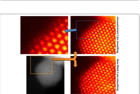
In all non-rigid registration approaches, there is one es-sential parameter that often receives little attention, that is, the transformation field smoothing kernel [18]. In this section, the effect of varying the size of this kernel is evaluated explicitly; it is compared with the‘row-locking’ alternative, and for the special case of loosely supported nanoparticles (that may rotate slightly with respect to the scan direction), a‘row-fitting’variant, Fig. 4.

Figure 4 exhibits several important trends, so we will begin by inspecting the unconstrained maps. The 5-pixel smoothed map clearly shows significant crystallographic information leaking into the diagnosis, the 2-pixel smoothing contains so many abrupt discontinuities it is unusable and even the 10-pixel smoothed map shows traces of lattice planes. This ‘leakage’of crystallographic information into the displacement field is a diagnosis artefact, and the fields required smoothing to at least 20 pixels to eliminate the lattice entirely. In all these plots, the outline of the nanoparticle is clearly visible and there

are several extreme ‘hot-spots’ around the perimeter

where significant transformations (relative to the refer-ence data) were diagnosed. These hot-spots correspond to atom positions that have moved or been sputtered through beam damage during the series, and such local-ised spatial transformations will significantly affect the image intensity data. We can also see bands similar to those in Fig. 3 running parallel to the fast-scan direction representing the genuine localised scanning distortions.

Applying the row-locking procedure yields the middle set of panels, and the similarities and differences be-tween these two approaches are important. Now, the sample edges and their associated artefacts are no longer present, nor signs of the sample crystallography, whilst the distortion bands parallel to the fast-scan direction are preserved. Again, we see that no longer relying on long-range smoothing of the transformation fields to eliminate artefacts allows a 2-pixel smoothed row-locked diagnosis to be used instead of a 40-pixel smoothed un-constrained diagnosis. This is important because the transformation fields should contain no sample or

Fig. 3Comparison of transformation field constraints diagnosed form an ADF time series of [100] MgO (y-direction shown only).Top-left, a simple 10-pixel Gaussian blurring;top-right, the row-locked equivalent. Note how the row-locked solution faithfully diagnoses the scanning distortions (horizontal bands) with no‘leakage’of the crystallographic structure. For completeness, the result of locking the rows across the slow-scan direction is shownbottom-left, indicating that the scanning distortions are not dominant along this direction. The reference image of the final iteration is shown for comparison.Colour scaleshows units of pixels, andgrey numbersindicate the total calculation time

crystallographic information at all. The instrumental dis-tortion exists with or without the presence of the sam-ple, so its diagnosis should not be dependent on it also. In theory, no smoothing could be used, but this small amount of 2 pixels improves robustness to shot noise.

A further key difference is observable between these and the unconstrained plots. The unconstrainedφyplots show a‘ramp’from left to right indicating that an add-itional affine transformation was present. The origin of this is small rotations of the loosely supported nanopar-ticle throughout the series, a problem which is difficult to avoid experimentally. Using the row-locked approach, these cannot be described, and hence, the sample rota-tion cannot be corrected. The solurota-tion to this is to use a constraint with an intermediate degree of restriction; here by fitting a low-order polynomial (linear in this case) to the fast-scan lines rather than simply locking them. This yields the third row of plots in Fig. 4. We now have transformation diagnosis, free from edge ef-fects and lattice artefacts but which can also diagnose and correct small sample rotations.

To quantify the sample rotation and its correction, lat-tice angles were measured throughout the image series using the point projective standard deviation technique (PPSD) [30]. Peak finding was first performed on each image (using the algorithm in [2]) to yield a sparse array

of points, and these were then Radon transformed and its standard deviation projected, Fig. 5. This PPSD measure-ment [30] reveals high-order crystallographic directions and is more sensitive to small changes in angle than the simple projective standard deviation measurement [5].

The PPSD analysis of the rigid-aligned data reveals a rotational range of approximately 2.8 °, Fig. 5. All lattice plane angles rotate equally indicating that this is a true rotation and not a shear. In the row-locked case, lattice angles close to 0 ° and 180 ° (parallel to the slow-scan direction) are well corrected but lattice planes near par-allel to the fast-scan direction are wholly uncorrected as expected. This is easily understood in terms of the

row-locking of the φy field which prevents image shear (or

rotation) along that direction.

For the row-fitted method, the PPSD analysis reveals full correction of sample rotation across all lattice orien-tations. If we recall the reference-updating iterative pro-cedure described above, the benefit of this rotation correction is further realised as the quality of the refer-ence image also improves greatly after just one iteration.

Whilst this hybrid method has proven useful for nano-particle time series registration, it should be noted that for more rigidly supported experimental samples, the more computationally efficient row-locking mode would be sufficient.

Fig. 6Enlargements from example non-rigid registration results corresponding to the transformation fields in Fig. 4.Top-rightunconstrained and

bottom-rightrow-fitted, both with 5-pixel smoothing.Top-left, a further enlarged view of the surface atoms with the unconstrained solution. Note the‘fish-eye’type distortions on the atomic columns in the bulk and the‘horse-tail’wispy elongations at the surface. All figures show the same colour scale

Fig. 5Lattice angles determined by PPSD analysis for the rigid-aligned data (top), and the row-locked (middle) and row-fitted (bottom) data.

Plotsshow the range 0 °–180 °

The artefact robustness of the row-locking/row-fitting procedure can be further inspected by comparing the re-sults against the unconstrained method at free sample edges. The same effect is true at sample defects and in-terfaces such as dislocations or grain boundaries. Figure 6 shows an extreme enlargement of the edge of the par-ticle analysed in Fig. 4.

The top-left edge of the nanoparticle at the free sur-face shows significant artefacts from the registration of the frame using unconstrained methods. The origin of this lies in the attempt to register the individual frame

to a reference that is the average frame. The result of this is that any genuine dynamic behaviour such as re-construction, damage or sputtering is corrupted in the process. The atomic columns in the centre of the par-ticle are also significantly distorted with a ‘fish-eye’ like appearance. This leads to a significant change in image intensity corrupting also any thickness or composition measurements.

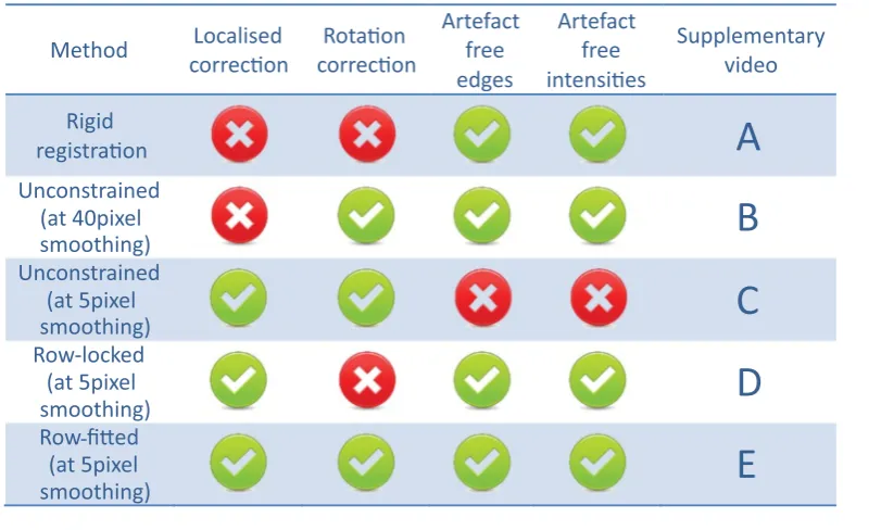
The performance of the various methods discussed are summarised in Table 1.

Summarising the results of Figs. 4 and 6 together in Table 1, we are left with a very powerful conclusion; it is impossible to define an unconstrained non-rigid transform-ation field that is both responsive to localised scanning

dis-tortions and free from artefacts. This problem is most

noticeable at free edges of samples, yielding significant im-plications for nanoscale strain mapping, and is likely to be the precision limiting factor in such investigations [31].

Algorithm optimisations and limitations

A number of further optimisations were developed alongside those above:

Choice of global or local reference frame

Iterative approach and convergence detection for improved computation speed

Restoration of secondary signals and Distortion frequency analysis

Choice of global or local reference image

In non-rigid registration, the choice of the reference image is crucial. In the accompanying code, two options are available to the user for choosing the non-rigid registra-tion reference data, either global reference or local refer-ence. In the case of an experimental time series (and in the absence of damage), we can assume the images are in-dependent viewings of the same underlying structure. Here, the mean through the already rigid registered image stack can be used as a suitable reference image. Alterna-tively, if the form of the image is changing through the series, such as an experimental STEM focal series, it is better to use the mean of the two neighbouring frames as the reference. This is suitable so long as the focal steps are finely enough sampled that no drastic change in the optical transfer function has occurred in the step. This neighbour average may also be more suitable if the experimental time series shows a significant

Table 1Performance evaluation of the rigid and non-rigid registration options discussed in the text

amount of sample change, say from electron-beam damage or dynamic surface refaceting.

Convergence detection for improved computation speed Within this nested iterative regime, the software is opti-mised to spend no longer than necessary performing each stage. To achieve this, an exit criterion has been added to the inner most loop (the distortion diagnosis) to exit when a certain precision of registration has been achieved. If the mean of the incremental offset maps falls below some certain threshold, we can say that the regis-tration has converged. In general, a value of 0.01 pixels represents a balance between computational speed and precision. In the accompanying code, the user may vary this parameter freely but is recommended not to go below 0.001 pixels as excessive computational time may result for no image quality benefit.

For high-throughput analysis of data algorithm, speed is clearly important. For the 512 × 512 pixel raw data shown in Figs. 3 and 4 with 31 and 57 frames, respectively (three passes, 0.01-pixel exit criterion), the total calculation times are shown alongside each condition. Generally, this was of the order of a few minutes. As an extreme test of the

MatLab™ code, a series of ten 4k STEM images (4096 ×

4096 pixel) were registered to an exit target of 0.05 pixels with three outermost update iterations. The total process-ing time was 1872 s (~31 min). For the STM data pre-sented later, the equivalent processing time was 66 s. All times correspond to an Intel™i7-870 at 2.93 GHz personal computer. Further speed improvements could likely be

realised if the MatLab™ code were migrated to a

multi-core or GPU deployment.

Restoration of secondary signals/spectral data

As the probe-sample interaction in the STEM generates several signals simultaneously, several data sets can be recorded simultaneously. In all cases, the same image/ sample drift relationship exists (rigid offsets) along with the same localised probe distortions (non-rigid offsets). In this way, multiple signals can be reregistered from the diagnosis performed on one. This secondary signal may be from another imaging detector, or equally x-ray or energy-loss spectral data. Where spectral data is being used, it is often of a far lower signal-to-noise ratio than the imaging data. This matching of the registration off-sets allows for the offoff-sets to be diagnosed from a high SNR data but applied to all.

Distortion frequency analysis

Image distortion is always best eliminated at source rather than via image processing. Previously, we have shown that analysis of offsets along the fast-scan direction allows for very high-frequency distortions, around 2 kHz, to be ana-lysed (see supplementary information of [2]). Extending the concept here to an analysis of the slow-scan rows, it is possible to analyse distortions of a very low frequency, around 0.2–3 Hz. Hopefully through such analysis, it is possible to identify the source of the distortion at its source in the EM suite, possible candidates at these low frequencies may be airflow or seismic vibrations.

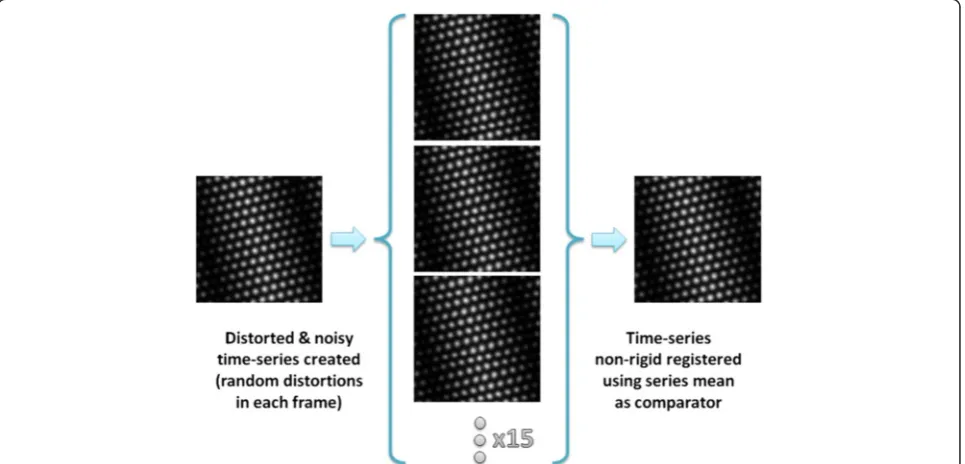
Fig. 7Stages in testing the fidelity of quantitative image intensity data, first creating distorted and noisy images (middle) before restoring them (right). Illustration shows crops from each stage, but a full-size version is included in the supplement

Limitations

One limitation of the gradient descent method that should be explicitly stated is that there exists the poten-tial to become ‘stuck’ in local minima. Without compu-tationally expensive multi-scale approaches [6], this cannot be avoided and imparts a practical consideration that the magnitude of any low-frequency scan distortion should not be larger than one half-unit cell within the size of the smoothing kernel range. If this is the case,

then, not only is image registration unsuitable but also it is not advised, as a distortion of this magnitude should really be resolved at an instrumental level. Fortunately, such large distortions are rarely observed, and computa-tionally efficient methods can be used.

Lastly, it should be noted that if the effects of kHz frequency distortions are very strong, these can persist even after correction as they are often strongly corre-lated along the fast-scan direction. Approaches to rotate

the acquisition will help make the appearance of these effects more isotropic [5], but ideally, these should be sought out at the environmental level.

Discussion

STEM ADF image intensity reliability

The so-called quantitative ADF makes use of image data recorded on an absolute scale and expressed in units of fractional beam intensity [32]. Using this method, it is pos-sible to count atoms either by comparison with simulation [33, 34] or by purely statistical methods [35]. However, in either case, it is the mean or integrated signal that is the metric used for comparison and this is susceptible to corruption by low-frequency scan distortion. These dis-tortions act to inflict a local change in magnification lead-ing to corruption of the quantitative signal.

To investigate this effect, simulated images of gold bi-wedges 1–12 atoms thick were deliberately distorted with

low-frequency sinusoids in both the x and y directions

similar to those observed experimentally (1 and 0.75 pixels peak-peak amplitude at 0.75 and 1.15 Hz, respectively) Fig. 7. Poisson-distributed image noise was also added to re-flect a realistic dose (105e−Å−2,≈1061 e−/pixel). This process was repeated over multiple crystal orientations (equivalent to STEM scan rotations) to avoid possible orientation bias. For each scan rotation, 15 images with unique distortions and noise were created as an analogue of an experimental time series. These time series were then non-rigid registered using the mean over all images as the reference data.

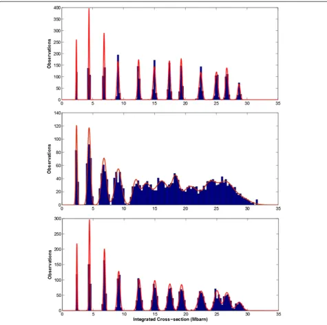
After registration, the scattering cross-sections of the atomic columns were calculated [34] and histograms of these are shown in Fig. 8. To each histogram, a Gaussian mixture fit was computed with 12 components so that

the mean and standard deviations of the cross-sections could be analysed [36].

Figure 8 (top) shows the clearly isolated peaks of the undistorted image. From this, we can conclude that for images whose performance is only limited by Poisson noise, we expect to be able to count atoms readily from the STEM image intensity using either simulation library or statistical methods [36]. Figure 8 (middle) shows the equivalent histogram after the introduction of scan dis-tortion. Here, we now see significant broadening and overlap of adjacent Gaussian components. For this dis-tribution, reservations would exist with atom-counting assignments greater than four atoms [37].

Following the restoration of the simulated time series, the first frame was taken and reanalysed. Importantly, to ensure a fair fixed-dose comparison, only the first frame of each series was analysed for the histograms. After res-toration, the Gaussians fitted to the histogram show a far narrower width (standard deviation) and therefore greatly reduced overlap. Here, atom-counting assign-ments would be accurately possible up to around nine atoms thickness, and reasonably reliable up to perhaps 12 atoms, a great improvement on the previous case.

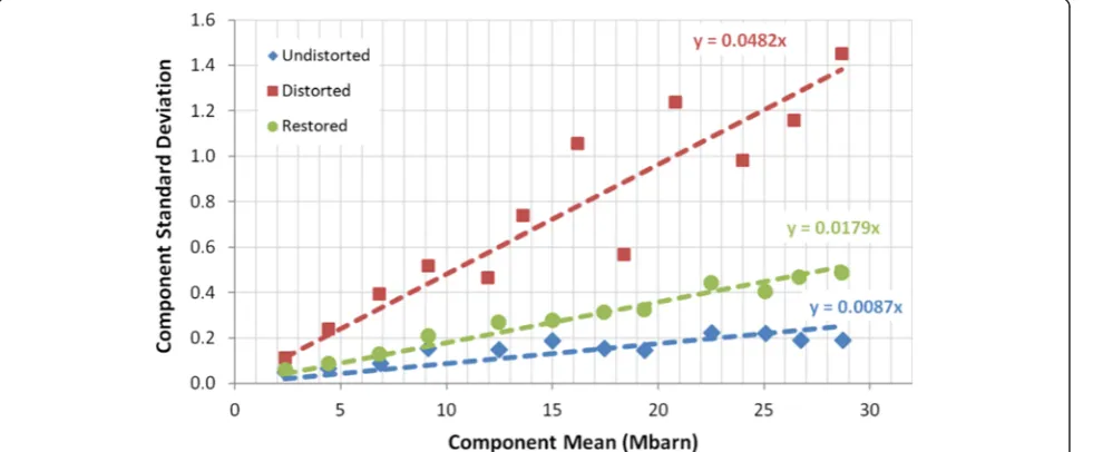
A more quantitative means to evaluate the importance of scan distortions in quantitative ADF is to examine the standard deviations of the 12 Gaussians fitted in Fig. 8, and these are shown in Fig. 9 (data table in Additional file 1). The overlap of neighbouring Gaussian compo-nents indeed defines the limits of atom counting with single-atom sensitivity [36–38].

First, considering the undistorted (as-simulated) images, we find that the standard deviation increases with the component mean. Here, a straight line has been fitted but for images dominated by Poisson noise only, we may have

Fig. 9Comparison of component mean and standard deviations from the histogram analysis in Fig. 8

expected a √mean relationship. Next, after inclusion of the scan distortion, we see that the standard deviation is increased by around a factor of 5. As Fig. 8 shows, this was improved after non-rigid registration with 77 % of the additional standard deviation now removed.

These results suggest that compensation of low-frequency scan distortion improves the fidelity of quanti-tative ADF image intensities leading to the potential to measure thickness or composition more accurately at atomic resolution. This need not necessarily demand any additional beam dose being required as previous work has shown that beam dose may be divided amongst a few experimental frames and these frames analysed col-lectively with equal accuracy [38]; in fact as demon-strated above, distortion compensation of a set of a few frames is likely to deliver a slightly improved precision over a single frame with the same total dose.

ADF image feature position reliability

In the previous section, we saw that the new non-rigid registration method can improve the reliability of the

integrated intensities of atomic columns. However, for many applications, such as structural or strain analyses, the positions of atomic columns are important and this is what is discussed here. Figure 6 shows how uncon-strained non-rigid transformation can corrupt the edge detail of nanoparticle samples, but the same could occur at interfaces within samples.

As describe above, non-rigid registration requires mul-tiple frames to operate and in this sense contains the re-dundant information necessary to separate the genuine sample data from the effects of distortion. When pre-sented with redundant or overdetermined data, statistical decomposition methods can also be used to extract the key varying components within the data set, such as prin-cipal component analysis (PCA) [39]. This is related to, but not the same as, noise filtering when used to describe all the information in a data set using the fewest number of principal components that contain meaningful informa-tion content.

In the example shown here, we use a [001] 6 ° sym-metric tilt grain boundary in strontium titanate SrTiO3

as an example. Fifty-two images were recorded along the grain boundary from which 212 dislocations were identi-fied to leave a set of cropped images. Although these dislocations are periodically spaced along the boundary plane, structural variations have been found in the core structures. Alternating dislocations have either a left- or right-handed nature depending on to which side the extra half-plane meets the next dislocation in the bound-ary (see Additional file 1: Figure S5); equally, we may ex-pect small variations in the occupancy of sites in the very centre of the core. Using these data, a PCA analysis

was performed using the MSA514 plug-in for ImageJ where the stack of images serve as the input.¹

Immediately upon producing the scree plot (see Additional file 1), differences can be seen between the rigid-only and the non-rigid registered data sets. The scree plots (Additional file 1: Figure S6) show reduced dimen-sionality of the non-rigid registered data. In the rigid-only

case, around twice as many components were required to describe the data above any given eigenvalue threshold (Fig. 10). To explore the differences further, the first few components for each case were plotted, Fig. 10 (larger ver-sions of these sub-plots are included in Additional file 1). In Fig. 10, the first six components are shown for the rigid-only case and the first three for the non-rigid, and beyond these components, no clear interpretation in terms of sample geometry was obvious and the images displayed mostly noise.

If we consider the component maps for the rigid-only case, we see that in many cases, the features show a po-larity, that is, there is a white and dark peak pair associ-ated with one another (compare with [4]). This translates to the component describing a shifting of the atomic column positions in the original images. How-ever, we have to be cautious with the interpretation of these component maps because of the way that STEM data is recorded. It has been shown previously that in the presence of image drift, the true form of the sample can be modified by some form of affine transformation [1–4]. Now, in the context of these affine transforms, let us look again at the first three components from the rigid-only set and the first component of the non-rigid set. In all of the first three components from the rigid-only set, we see a band through the centre of diffuse grey, that is of little significance. Above and below this mid-line, we see two distinctly different behaviours in

the feature polarity (real-image feature shift). The first and third components exhibit a shearing-type behaviour inclined at 45 ° from the horizontal and 90 ° from one another; the second again shows a similar shearing-type behaviour but now roughly parallel to the fast-scan (horizontal) direction. These displacements are in fact the result of image drift and/or scan distortion. The ob-servant reader may wonder why there is not a fourth shearing-type component perpendicular to the second and this will be discussed later. These three distorted components are shown alongside the first component from the corrected data set. In fact, if the vectors shown on the rigid-only maps 1–3 are added together, they will close and yield minimal overall displacement. This result is consistent then with the first corrected component

showing almost no polarity—it merely shows the

vari-ation from the mean of the white atomic columns and dark dislocation core.

The next comparable components are the fourth rigid-only and the second non-rigid; here, we see a compo-nent that describes the correlation between an increased occupancy of the terminating half-plane with an outward displacement of the adjacent planes. This is consistent with elastic theory and offers a useful route to studying this occupancy-strain relationship.

Lastly, the fifth and sixth components of the rigid-only data set and the third component of the non-rigid are closely comparable. In this component, we see the effect of

Fig. 11aAn example frame from an STM image series of SrTiO3(001) trilines [41] (field of view = 40 × 40 nm2_{) andbthe restored image from} the frame series.Line profilescorrespond to the regions indicated by thewhite lines. Note that both the tip-height artefacts (horizontal bright/dark bands) as well as the lateral distortions have been corrected. The periodicity along the ridge of the triline (≈2 Å spacing) is directly interpretable after restoration

the previously mentioned left- or right-handedness of the staggered dislocations. Unfortunately, this useful genuine information has become conflated in the rigid-only case with the fourth and final image drift distortion described earlier. Now, in the presence of image drift, another add-itional component becomes necessary to describe this combination of the displacements and image drift.

Application to scanning tunnelling microscopy

The methods demonstrated for registering STEM data are equally applicable to other scanned probe microscopies such as atomic force microscopy (AFM) or scanning tun-nelling microscopy (STM) where careful image reregistra-tion is equally important. Here, thermal drift is again problematic [40] and this can often be corrected using af-fine transformations [3]. Again, the same prior knowledge regarding the fast-scan behaviour can be utilised to im-prove the registration performance and using the robust ‘row-locking’ technique, it is possible to perform robust non-rigid registration capable of outperforming the more restrictive affine or polynomial unwarping.

To demonstrate this, an example STM time series data set was registered (original data set details as in [41]). The registration of scanned physical, as opposed to elec-tron, probe microscopy is complicated by one additional factor—that of tip-height artefacts. This manifests itself as regions of brighter and darker bands representing the temporary offset in the height of the scanning tip (or bright/dark rings in a spiral scan [16]). Again, as for lateral distortions this is heavily correlated along the fast-scan dir-ection and can be corrected as such [15]. To correct for tip-height errors, the data was rigid registered, and then, the median height was calculated row-wise. For each image, this was then corrected to be brought to the mean of the median heights over the whole of the image series. After this height correction, the data were non-rigid registered using the‘row-locking’feature described earlier; the result of correcting the data series is shown in Fig. 11. A movie of the raw and registered data is provided in Additional files 2, 3, 4, 5, 6, 7 and 8. The reader may wish to compare these with the manual registration performed previously and available in the supplementary data of [41].

After correction of the tip-height and low-frequency lateral distortions, it is possible to either play back the movie of the data (see Additional files 2, 3, 4, 5 and 6) and view the dynamic processes without distraction or to average through the image series to improve signal-to-noise ratio (SNR) for improved measurement preci-sion (Fig. 11b).

Conclusions

A single serial-acquired image (STEM, STM, AFM etc.) combines genuine sample information and the effects of

possible scanning distortions. Recording multiple frames of serial-acquired data yields a separable data set with information about both the sample and any scanning distortions which can be diagnosed and corrected by non-rigid registration. In experimental data, scanning distortions were found to be highly correlated along a fast-scan row, but far more varying between rows (in the slow-scan direction). This phenomenological description was used to design new‘row-locked’and‘row-fitted’ dis-tortion field constraints that alleviate the need for long-range smoothing kernels. These approaches were tested and found to deliver more localised image correction without the introduction of artefacts at sample edges or interfaces.

The distortion correction technique was tested in three case studies: ADF intensity quantification, interface structural interpretation and STM resolution/SNR. In all cases, the precision and interpretability of the data were improved. Further optimisation of the improvement in ADF intensity- and strain-precision as a function of the scan speed, electron dose and optimum number of frames is an ongoing study. The software described in this work is available free of charge for academic/non-commercial use from www.lewysjones.com.

Endnote

1

Plug-in details can be found at: http://rsb.info.nih.gov/ ij/plugins/inserm514/Documentation/MSA_514/MSA.html

Additional files

Additional file 1:Supplementary information.Additional information, details of pure noise artifact testing, and enlargements of some figures.

Additional file 2:Video A.Rigid registered only ADF time-series. Additional file 3:Video B.Unconstrained non-rigid registration result with 40 pixel smoothing range.

Additional file 4:Video C.Unconstrained non-rigid registration result with 5 pixel smoothing range.

Additional file 5:Video D.Row locked' non-rigid registration result with 5 pixel smoothing range.

Additional file 6:Video E.'Row fitted' non-rigid registration result with 5 pixel smoothing range.

Additional file 7:Raw STM Data.Unprocessed STM raw data. Additional file 8:Registered STM Data.STM data after tip-height correction and rigid and non-rigid registration.

Competing interests

The authors declare that they have no competing interests.

Authors’contributions

Acknowledgements

The authors would like to acknowledge Prof. Yuichi Ikuhara for providing the bi-crystal grain boundary specimen which was imaged at the EMSL, a national scientific user facility sponsored by the Department of Energy’s Office of Biological and Environmental Research and located at PNNL. We acknowledge Dirk-Jan Kroon for his submission on the MatLab File Exchange which proved some initial insights and Gerardo Martinez and Annick De Backer (EMAT Antwerp) for providing the simulation of the platinum wedge and helping fit the GMM distribution shown in Fig. 8. The research leading to these results has received funding from the EU FP7 (grant agreement 312483-ESTEEM2, Integrated Infrastructure Initiative–I3), the UK EPSRC (grant number EP/K032518/1), the US DoE (grant number DE-FG02-03ER46057) and the Chemical Imaging Initiative at PNNL under contract DE-AC05-76RL01830 operated for DoE by Battelle.

Author details

1_{Department of Materials, University of Oxford, Oxford, UK.}2_EPSRC

SuperSTEM Facility, Daresbury Laboratory, Warrington, UK.3Department of Applied Physics, Yale University, New Haven, CT, USA.4_{EMAT, University of} Antwerp, Antwerp, Belgium.5Physical Sciences Division, Pacific Northwest National Laboratory, Richland, WA, USA.

Received: 7 April 2015 Accepted: 3 June 2015

References

1. Recnik, A, Möbus, G, Sturm, S: IMAGE-WARP: a real-space restoration method for high-resolution STEM images using quantitative HRTEM analysis. Ultramicroscopy.103(4), 285–301 (2005)

2. Jones, L, Nellist, PD: Identifying and correcting scan noise and drift in the scanning transmission electron microscope. Microsc. Microanal. 19, 1050–1060 (2013)

3. Rahe, P, Bechstein, R, Kühnle, A: Vertical and lateral drift corrections of scanning probe microscopy images. J. Vac. Sci. Technol. B Microelectron. Nanom. Struct.28, C4E31 (2010)

4. Kimoto, K, Asaka, T, Yu, X, Nagai, T, Matsui, Y, Ishizuka, K: Local crystal structure analysis with several picometer precision using scanning transmission electron microscopy. Ultramicroscopy.110(7), 778–782 (2010) 5. Sang, X, LeBeau, JM: Revolving scanning transmission electron microscopy: correcting sample drift distortion without prior knowledge. Ultramicroscopy. 138C, 28–35 (2013)

6. Sun, Y, Pang, JHL: AFM image reconstruction for deformation measurements by digital image correlation. Nanotechnology. 17(4), 933–9 (2006)

7. Berkels, B, Binev, P, a Blom, D, Dahmen, W, Sharpley, RC, Vogt, T: Optimized imaging using non-rigid registration. Ultramicroscopy.138, 46–56 (2014) 8. Sanchez, AM, Galindo, PL, Kret, S, Falke, M, Beanland, R, Goodhew, PJ: An approach to the systematic distortion correction in aberration-corrected HAADF images. J. Microsc.221(Pt 1), 1–7 (2006)

9. Braidy, N, Le Bouar, Y, Lazar, S, Ricolleau, C: Correcting scanning instabilities from images of periodic structures. Ultramicroscopy.118, 67–76 (2012) 10. Marinello, F, Carmignato, S, Voltan, A, Savio, E, De, L: Chiffre Error sources in

atomic force microscopy for dimensional measurements: taxonomy and modeling. J. Manuf. Sci. Eng.132(3), 030903 (2010)

11. Shatsky, M, Hall, RJ, Brenner, SE, Glaeser, RM: A method for the alignment of heterogeneous macromolecules from electron microscopy. J. Struct. Biol. 166(1), 67–78 (2009)

12. Kuglin, CD, Hines, DC: The phase correlation image alignment method. Proc. Int. Conf. Cybern. Soc.1975, 163–165 (1975)

13. van Heel, M, Schatz, M, Orlova, E: Correlation functions revisited. Ultramicroscopy.46, 307–316 (1992)

14. Zitová, B, Flusser, J: Image registration methods: a survey. Image. Vis. Comput. 21(11), 977–1000 (2003)

15. Anguiano, E, Aguilar, M: A cross-measurement procedure (CMP) for near noise-free imaging in scanning microscopes. Ultramicroscopy.76, 39–47 (1999) 16. Wang, JJ, Hou, Y, Lu, Q: Self-manifestation and universal correction of image

distortion in scanning tunneling microscopy with spiral scan. Rev. Sci. Instrum.81(7), 3–8 (2010)

17. Yu, L, Zhang, D, Holden, E-J: A fast and fully automatic registration approach based on point features for multi-source remote-sensing images. Comput. Geosci.34(7), 838–848 (2008)

18. Cachier, P, Pennec, X, Ayache, N: Fast non rigid matching by gradient descent: study and improvements of the‘Demons’algorithm. (1999) 19. Wang, H, Dong, L, O’Daniel, J, Mohan, R, Garden, AS, Ang, KK, Kuban, DA,

Bonnen, M, Chang, JY, Cheung, R: Validation of an accelerated‘demons’ algorithm for deformable image registration in radiation therapy. Phys. Med. Biol.50(12), 2887–905 (2005)

20. Mao, Y, Gilles, J: Non rigid geometric distortions correction-application to atmospheric turbulence stabilization. Inverse. Probl. Imaging. 1–15 (2012). 21. Pennycook, TJ, Jones, L, Pettersson, H, Coelho, J, Canavan, M,

Mendoza-Sanchez, B, Nicolosi, V, Nellist, PD: Atomic scale dynamics of a solid state chemical reaction directly determined by annular dark-field electron microscopy. Sci. Rep.4, 7555 (2014)

22. Jones, L, MacArthur, KE, Fauske, VT, van Helvoort, ATJ, Nellist, PD: Rapid estimation of catalyst nanoparticle morphology and atomic-coordination by high-resolution z-contrast electron microscopy. Nano. Lett.14(11), 6336–41 (2014)

23. Sawada, H, Watanabe, M, Chiyo, I: Ad hoc auto-tuning of aberrations using high-resolution STEM images by autocorrelation function. Microsc. Microanal.18(4), 705–10 (2012)

24. Jones, L, Nellist, PD: Testing the accuracy of the two-dimensional object model in HAADF STEM. Micron.63, 47–51 (2014)

25. Martinez, GT, Jones, L, De Backer, A, Béché, A, Verbeeck, J, Van Aert, S, Nellist, PD: Quantitative STEM normalization: the importance of the electron flux. Ultramicroscopy. vol. [submitted, 2015]

26. Padowitz, DF, Hamers, RJ: Voltage-dependent STM images of covalently bound molecules on Si(100). J. Phys. Chem. B.102(100), 8541–8545 (1998) 27. Kroon, D, Slump, C: MRI modality transformation in demon registration.

Imaging from nano to macro.2(3), 3–6 (2009)

28. Couillard, M, Radtke, G, Botton, GA: Strain fields around dislocation arrays in a S9 silicon bicrystal measured by scanning transmission electron microscopy. Philos. Mag.93(10–12), 1250–1267 (2013)

29. Zuo, J-M, Shah, AB, Kim, H, Meng, Y, Gao, W, Rouviére, J-L: Lattice and strain analysis of atomic resolution Z-contrast images based on template matching. Ultramicroscopy.136, 50–60 (2014)

30. Sang, X, Oni, Aa, Lebeau, JM: Atom column indexing: atomic resolution image analysis through a matrix representation. Microsc. Microanal. 1–8 (2014)

31. Yankovich, AN, Berkels, B, Dahmen, W, Binev, P, Sanchez, SI, Bradley, SA, Li, A, Szlufarska, I, Voyles, PM: Picometre-precision analysis of scanning transmission electron microscopy images of platinum nanocatalysts. Nat. Commun.5, (2014)

32. LeBeau, JM, Stemmer, S: Experimental quantification of annular dark-field images in scanning transmission electron microscopy. Ultramicroscopy. 108(12), 1653–1658 (2008)

33. LeBeau, JM, Findlay, SD, Allen, LJ, Stemmer, S: Standardless atom counting in scanning transmission electron microscopy. Nano. Lett.10(11), 4405–8 (2010) 34. MacArthur, HEKE, Pennycook, T, Okunishi, E, D’Alfonso, AJJ, Lugg, RR, Allen, LJ, Nellist, PD: Probe integrated scattering cross sections in the analysis of atomic resolution HAADF STEM images. Ultramicroscopy.133, 109–19 (2013) 35. Van Aert, S, Batenburg, KJ, Rossell, MD, Erni, R, Van Tendeloo, G:

Three-dimensional atomic imaging of crystalline nanoparticles. Nature.470(7334), 374–7 (2011)

36. De Backer, A, Martinez, GT, Rosenauer, A, Van Aert, S: Atom counting in HAADF STEM using a statistical model-based approach: methodology, possibilities, and inherent limitations. Ultramicroscopy.134, 23–33 (2013) 37. Van Aert, S, De Backer, A, Martinez, GT, Goris, B, Bals, S, Van Tendeloo, G, Rosenauer, A: Procedure to count atoms with trustworthy single-atom sensitivity. Phys. Rev. B-Condens Matter Mater. Phys.87(6), 1–6 (2013) 38. De Backer, A, Martinez, GTT, MacArthur, KE, Jones, L, Béché, A, Nellist, PD,

Van Aert, S, De Backer, A, Martinez, GTT, MacArthur, KE, Jones, L, Béché, A, Nellist, PD, Van Aert, S: Dose limited reliability of quantitative ADF STEM for nano-particle atom-counting. Ultramicroscopy.151, 56–61 (2015) 39. Wold, S, Esbensen, K, Geladi, P: Principal component analysis. Chemom.

Intell. Lab. Syst.2(1–3), 37–52 (1987)

40. Marinello, F, Balcon, M, Schiavuta, P, Carmignato, S, Savio, E: Thermal drift study on different commercial scanning probe microscopes during the initial warming-up phase. Meas. Sci. Technol.22, 094016 (2011) 41. Marshall, MSJ, Becerra-Toledo, AE, Marks, LD, Castell, MR: Surface and defect

structure of oxide nanowires on SrTiO 3. Phys. Rev. Lett.107(8), 086102 (2011)