Analysis of colour constancy algorithms using the knowledge of variation of correlated colour temperature of daylight with solar elevation

(1)

R E S E A R C H

Open Access

Analysis of colour constancy algorithms using the

knowledge of variation of correlated colour

temperature of daylight with solar elevation

Sivalogeswaran Ratnasingam

1,3,4*

, Steve Collins

1

and Javier Hernández-Andrés

2

Abstract

In this article, we present an investigation of possible improvement of the colour constant reflectance features that can be obtained from daylight illuminated scenes using pixel-level colour constancy algorithms (model-based algorithm: S Ratnasingam, S Collins, J. Opt. Soc. Am. A27, 286–294 (2010) and Projection-based algorithm: GD Finlayson, MS Drew, IEEE ICCV, 2001, pp. 473–480). Based on the investigation we describe a method to improve the performance of the colour constancy algorithms using the correlation between the correlated colour

temperature of measured daylight with the solar elevation and phase of the day (morning, midday and evening). From this observation, the data from 1 year are used to create a solar elevation and phase of day-dependant method of interpreting the information obtained the colour constancy algorithms. Test results show that using the proposed method with 40-dB signal-to-noise ratio the performance of the projection-based algorithm and model-based algorithm can be improved on average by 33.7 and 45.4%, respectively. More importantly, a larger

improvement (85.9 and 113.7%) was obtained during the middle period of each day which is defined as when the solar elevation is larger than 20°.

Keywords:Colour constancy, Illuminant invariant chromaticity

1. Introduction

Colour is a useful feature in several machine vision appli-cations including object recognition and image indexing. However, the apparent colour of an object varies depen-ding on the viewing environment, particularly in scenes illuminated by daylight. Colour-based recognition in na-turally illuminated scenes is therefore a difficult problem and existing techniques are not effective in real scenes [1-6]. The problems with obtaining colour information from naturally illuminated outdoor scenes arise from the uncontrolled changes to both the intensity and the spec-tral power distribution of daylight. The resulting variations in the recorded colour of the same object under different daylight conditions make it difficult to use colour as a reliable source of information in machine vision applica-tions [3-6].

In contrast to camera-based systems, the human visual system’s perception of the colour of an object is largely independent of the illuminant. Several approaches to replicating the colour constancy achieved by the human visual system have been proposed [6]. However, many of these algorithms assume that scene is illuminated uni-formly and shadows mean that this assumption is not always valid for outdoor scenes. The assumption that a scene is uniformly illuminated is avoided by those colour constancy algorithms that only use pixel-level informa-tion. Marchant and Onyango [7], Finlayson and Hordley [8] and Romero et al. [9] have all proposed methods for obtaining a single illuminant invariant feature from pixel data under daylight based on the assumptions that the spectral responses of the sensors are infinitely narrow and that the power spectral density of the illuminant can be approximated by the power spectral density of a blackbody illuminant. However, a single feature poten-tially leads to confusion between some perceptually dif-ferent colours [6]. This confusion can be avoided using the method proposed by Finlayson and Drew [10] that * Correspondence:[email protected]

1_{Department of Engineering Science, University of Oxford, OX1 3PJ Oxford,}

UK

3_{The Australian National University, Canberra ACT 0200, Australia}

Full list of author information is available at the end of the article

(2)

obtains two illuminant independent features from the responses of four sensors with different spectral res-ponses. Based on the same assumptions of infinitely narrow band sensors and the blackbody model of the illuminant, Ratnasingam and Collins [11] proposed a sim-ple method of obtaining two illuminant independent features from the responses of four sensors. Since neither of the assumptions upon which all these methods is strictly applicable, Ratnasingam and Collins [11] also pro-posed a method for determining the quality of the spectral information that can be obtained from the features ob-tained using these methods. One important conclusion from their work was that pixel-level colour constancy algorithms extract useful information from the responses of sensors whose spectral response covers a wavelength range of 80 nm or less [11]. Subsequently, Ratnasingam et al. [12] investigated the possibility of optimising the spectral responses of the image sensors to improve the quality of the illuminant invariant features that can be obtained from daylight illuminated scenes using pixel-level colour constancy algorithms. The conclusion of this study was that the widely available International Commis-sion on Illumination (CIE) standard illuminants was not representative enough to the actual daylight measure-ments obtained under widely varying weather conditions to be used to reliably optimise the spectral responses [12].

Studying the pattern of variation of the daylight spec-tra would be very useful because daylight dominates in the day time and some important machine vision appli-cations, including remote sensing, controlling unmanned vehicles and simultaneous localisation and mapping, are based upon processing outdoor scenes. The variation in spectral power distribution of the daylight due to the variation in solar elevation, time of year and geographic location leads to difficulties in reliably recognising ob-jects or scenes. In this article, we investigate the advan-tages of using solar elevation and phase of the day as auxiliary information to enhance the performance of a colour constancy algorithm. This auxiliary information can be calculated if the time of day, date and the geo-graphic location of the camera are known. However, it is difficult to model such a relation with the artificial illuminants. But, one could use the knowledge of whether the scene is indoor or outdoor to account for the illuminant in these scenarios. Based on this evidence an approach for improving the performance of colour constancy algorithms that can be obtained from daylight illuminated scenes is proposed based upon the observed variation of the correlated colour temperature (CCT) of measured daylight with solar elevation and date. Here, it is worth noting that in our investigation for possible improvement of colour constancy algorithms we only use the approximate geographic location (example country or region) and phase of the day (i.e. morning, midday and

afternoon) as auxiliary information to the colour con-stancy algorithms. The performance improvement ob-tained using the proposed approach has been illustrated using two existing colour constancy algorithms proposed by Finlayson and Drew [10] and that proposed by Ratnasingam and Collins [11]. Here, we should note that the algorithms chosen to investigate the performance enhancement of colour constancy using solar elevation and date, do not rely on the content of the rest of the scene in extracting the illuminant invariant features. This choice was made because outdoor scene might consist of regions illuminated by direct sunlight or skylight or under shadow and the power spectrum of the incident light in these regions will not be the same [13]. This means in the outdoor scenes where the intensity and the relative power spectrum vary spatially, the performance of any algorithm that processes the entire scene to obtain an estimate for the illuminant, significantly degrades in any real-world scenes therefore not appropriate for machine vision appli-cations. For this reason, we have chosen two algorithms that extract illuminant invariant features at pixel level rather than processing the whole scene.

The remainder of this article is organised as follows: In Section 2, a brief description of the algorithm of obtaining useful features related to the reflectance of a surface proposed by Finlayson and Drew [10] and Ratnasingam and Collins [11] is presented. In Section 3, a description of the proposed method for improving the degree of illuminant invariance obtained from the fea-tures determined using the two different methods is given. Simulation results to assess the effectiveness of the proposed method are then presented in Section 4. Finally, Section 5 contains the conclusions of this study.

2. Descriptions of the algorithms and assessment method

When the incident light Ex(λ) reflects on an object’s surface at point x with reflectance spectrum Sx(λ) the image sensor responseRx,Ecan be given by

Rx;E¼ix:jxIx

Z

ω

Sxð Þλ Exð Þλ Fð Þλ dλ ð1Þ

whereF(λ) is the spectral sensitivity of the image sensor andIxis the intensity of the incident light at scene point x. The unit vectors ix and jx denote the directions of

the illuminant and the surface normal, respectively. The dot product between these two unit vectors ix

:jx

(3)

Rx;E¼ix:jxIxSxð Þλi Exð Þλi ð2Þ

To make the product of terms on the right-hand side of Equation (2) into simple summation, we take natural logarithm to both sides of Equation [10,11].

logRx;E_¼_log_f_Gx_Ix_{g þ}_log _Ex _λ i

ð Þ

f g þlog Sx _λ i

ð Þ

f g; ð3Þ

where Gx(=ix.jx) is the geometry factor. On the right-hand side of the above equation, the first term (GxIx) depends on the geometry of the scene and illuminant intensity. The second term (Ex(λi)) depends only on the

relative power spectrum of the illuminant and the third term (Sx(λi)) depends only on the reflectance of the

object’s surface. From this one can understand that for obtaining scene independent perceptual descriptors we need to remove the first two components. Moreover, the first term can be removed by taking the difference between two image sensor responses that have different spectral sensitivities. Once the scene geometry compo-nent and intensity compocompo-nents have been removed the only scene dependent term is the power spectrum of the illuminant. This could be removed by assuming a para-metric model for the illuminant power spectrum. Based on this, Finlayson and Drew [10] proposed an algorithm for colour constancy based on the assumptions that the spectral power distribution of the illuminant can be modelled by Wien’s radiation law. To remove the changes in the power spectral density of the illuminant from the log-difference features, Finlayson and Drew used eigen vector decomposition and projected the three log-difference features in the direction of largest eigen vector. This resulted in a two-dimensional space where a reflec-tance can be located approximately invariant to illumi-nant. To find the relevant eigen vectors, Finlayson and Drew used 18 non-grey patches of the Macbeth Colour Checker chart and blackbody illuminants with colour temperatures between 5,500 and 10,500 K. As the black-body model of illuminant is not the most appropriate model for real-world illuminants we adapted Finlayson and Drew’s algorithm to improve in such a way that we used the CIE standard [14] representing the daylight at different phase of the day and the standard Munsell reflectance data base [15] for obtaining more realistic estimation of the direction of illuminant induced variation. In the remainder of the article, we refer to this adapted version of the algorithm as the projection algorithm. Once we have estimated the more realistic direction of illumi-nant-induced variation using eigen vector decomposition we projected the logarithm difference features in that direction and obtained two features that are invariant to illuminant, and scene geometry. The two illuminant invariant features (F1Proj and F2Proj) from the

projection-based algorithm were obtained as follows:

F1Proj¼LogDiff;Eig1 ð4Þ

F2Proj¼LogDiff;Eig2 ð5Þ

where LogDiff= [log (R2)−log (R1), log (R3)−log (R1), log

(R4)−log (R1)] and 〈 〉 means scalar product. The

quan-titiesR1,R2,R3andR4are the sensor responses numbered

from the shortest wavelength end of the spectrum and

Eig1andEig2are the two smallest eigen vectors obtained

from the eigen vector decomposition applied on the normalised sensor responses.

The other algorithm that we investigated is the rela-tively simple algorithm proposed by Ratnasingam and Collins [11]. This algorithm is also based on the black-body illuminant model and infinitely narrow band sensor assumptions in deriving two illuminant invariant reflec-tance features from four sensor responses (referred to in this article as the model-based algorithm). As opposed to Finlayson and Drew’s [10] algorithm, Ratnasingam and Collins’[11] algorithm processes three adjacent sen-sor responses to obtain an illuminant invariant feature. In particular, if we number the image sensor responses as R1, R2, R3 and R4, the model-based algorithm

mates an illuminant invariant reflectance feature by esti-mating the illuminant effect on the sensor response R2

using the sensor responsesR1andR3. Similarly, a second

illuminant invariant reflectance feature is extracted by estimating the illuminant effect on the sensor response R3using the sensor responses R2and R4. The two

illu-minant invariant reflectance features (F1Modeland F2Model)

are obtained as follows:

F1Model¼logð Þ R2 fαlogð Þ þR1 ð1αÞlogð ÞR3 g ð6Þ

F2Model¼logð Þ R3 fγlogð Þ þR2 ð1γÞlogð ÞR4 g ð7Þ

whereαandγare two parameters referred to as channel coefficients. Ifλ1,λ2,λ3andλ4are the peak wavelengths

of the four image sensors the two features are ideally independent of the illuminant if the two channel coeffi-cients are chosen so that the following two equations are satisfied [11].

1 λ2

¼ α λ1

þ1α λ3

ð8Þ

1 λ3

¼ γ λ2

þ1γ λ4

ð9Þ

(4)

of the four image sensors evenly across the visible spectrum, 400–700 nm, and the spectral full width at half maximum of 80 nm was chosen to have approximately the same width as consumer cameras (Sony DXC930). The channel coefficients (α and γ) were obtained by the optimisation process described by Ratnasingam et al. [12]. The channel coefficients listed in Table 1 are the optimum values that give the best illuminant invariant reflectance features. The two eigen vectors listed in Table 2 are the two smallest vectors obtained by applying eigen vector decomposition on the logarithm difference of the sensor responses generated by the 100 pairs of Munsell samples (1 CIELab unit pair wise distance) when illuminated by the 20 spectra of CIE standard illuminants.

The results in Figure 1 show that, except for a region of metamers (metamers for F1Model and F2Model space),

different colours are projected to different parts of this feature space. Previously, the results obtained from the same Munsell reflectances when illuminated by CIE standard daylight with different CCTs showed that a residual illuminant dependency causes small variations in the projected position of each reflectance sample in the feature space [11].

As the model-based and projection-based algorithms extract features that are independent of the lightness component of a colour, the performance of these two algorithms have been investigated using three sets of 100 pairs of reflectances chosen from normalised Munsell reflectance spectra [12]. As described by Ratnasingam et al. [12], each of these three test reflectance sets has 100 pairs of reflectances with pair wise distances of either 0.975 to 1.025 CIELab units, 2.99 to 3.01 CIELab units or 5.995 to 6.005 CIELab units, respectively. These three sets were chosen based on the colourimetric description of the CIELab space. In the CIELab space, colours separated by less than 1 unit are described as not perceptibly different, 1–3 units are as very good match to each other and 3–6 units as a good match for an average person [16]. These colourimetric descriptions have widely been used by researchers in colourimetric experiments [16-18]. Even though differences of 1 CIELab unit are described as not perceptible by an average human observer [18] we have included this data in the test set to investigate if the proposed algorithm is better than the human visual system in recognising perceptually similar colours. In fact our results show that the algorithm can differentiate more than 25% of the pairs of ‘colours’that are described as not perceptibly different to an average human.

To investigate both the algorithms in more realistic circumstances the sensor noise was modelled as described by Ratnasingam and Collins [11]. Particularly, 30 and 40 dB signal-to-noise ratio (SNR) was considered in this investigation and the resultant responses were quantised with a 10-bit quantiser [12]. The features extracted from the simulated noisy sensor responses to a particular reflectance spectrum when it is illuminated by daylight spectra with different CCTs form a cluster of points in the two-dimensional feature spaces. These clusters arise be-cause of a combination of the differences between the power spectral densities of daylight and those of black-bodies, finite spectral sensor width and the noisy sensor responses. To investigate the relative significance of these two factors, the features extracted from 1,269 Munsell

-0.6 -0.4 -0.2 0 0.2 0.4 0.6 0.8

-0.2 -0.1 0 0.1 0.2 0.3 0.4 0.5 0.6

F 1 Model

F2

Model

Figure 1Illuminant independent feature space formed by model-based algorithm using 202 Munsell samples and the CIE D65 illuminant.

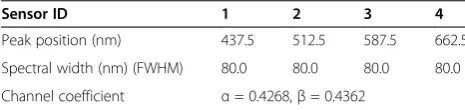
Table 1 The wavelengths corresponding to the peak sensor responses and full width half maximum (FWHM) of the spectral responses of sensors with Gaussian spectral responses used to investigate both the model-based and projection-based algorithms

Sensor ID 1 2 3 4

Peak position (nm) 437.5 512.5 587.5 662.5

Spectral width (nm) (FWHM) 80.0 80.0 80.0 80.0

Channel coefficient α= 0.4268,β= 0.4362

The table also contains the channel coefficients for the model-based algorithm [11].

Table 2 The wavelengths corresponding to the peak sensor responses and FWHM of the spectral responses of sensors with Gaussian spectral responses used to investigate the projection-based algorithm

Sensor ID 1 2 3 4

Peak position (nm) 437.5 512.5 587.5 662.5

Spectral width (nm) (FWHM) 80.0 80.0 80.0 80.0

Eigen vector 1 0.0977 0.366–0.925

Eigen vector 2 0.647–0.729–0.220

(5)

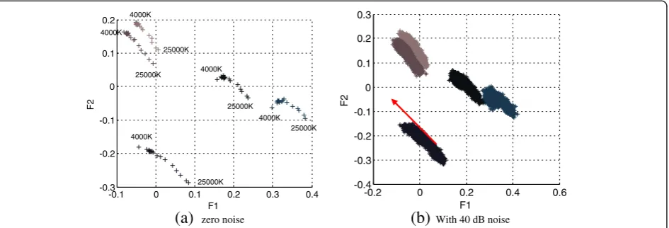
samples were compared. When ‘illuminated’ by 20 CIE daylight spectra all the colours exhibited a behaviour simi-lar to the behaviour shown by the five representative Munsell reflectances (Munsell samples: 2.5R 9/2, 5YR 6/10, 10Y 9/10, 5 PB 2.5/1 and 10P 4/1) shown in Figure 2. In particular, it was found that on average when the SNR is 40 dB the variation caused by the residual illuminant dependence is three times larger in a particular direction (see Figure 2b) compared to the variations caused by the sensor noise. More importantly, the residual illuminant dependency causes variation mainly in one direction and the sensor noise shows a Gaussian distribution. This observation suggests that if any information related to the probable illuminant spectrum is available then it might be possible to improve the interpretation of the features obtained from a pixel-level colour constancy algorithm.

3. Proposed approach for improving colour constancy

The Sun is the dominant natural light source during the day. The power spectral density of the sunlight above the Earth’s atmosphere can be approximated by the spec-trum of a blackbody. However, this is only an approxima-tion and the spectral peak wavelength, 475 nm, is the same as the peak wavelength for a blackbody with colour temperature 6,101 K, whilst taking into account the entire spectrum the CCT is 5750 K [19]. To reach the Earth’s surface this light must travel through the atmosphere where it is both scattered and absorbed. The path length of the light from the edge of the atmosphere to the Earth’s surface depends upon the angle of elevation between the horizon and the Sun’s position in the sky. As a result the

CCT of the daylight reaching the surface of the Earth is expected to depend upon the solar elevation.

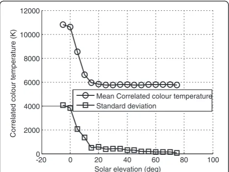
The relationship between the CCT of measured day-light spectra and either the solar elevation or the time of day has been investigated using daylight spectra mea-sured over a 2-year period (1996 and 1997) in Granada, Spain [20]. Over the 2-year period, 2,600 daylight spectra were measured at approximately hourly intervals and the time at which each spectrum was measured was recorded using GMT. In particular, these spectral measurements were taken in different seasons, different weather conditions and also under direct sunlight, skylight and with the Sun behind clouds. Figure 3 shows the mean variation and standard deviation of CCT of measured daylight with elevation. These results show that the CCT of the daylight is approximately 5,750 K during the middle of the day and during this period the standard deviation of the CCT values is relatively low. In contrast, just after sunrise and just before sunset the mean value of CCT of the daylight increases and the standard deviation also increases (see Figure 3). The important ob-servation from the data in Figure 3 is that using solar elevation information to influence the interpretation of the outputs from colour constancy algorithms might im-prove the results obtained. The solar elevation can be cal-culated from the location of a camera and the time of the day [21].

The path length of the light through the atmosphere is only one of the factors that determine the amount of scattering and absorption that will occur at a particular moment. Moreover, the amount of absorption and scat-tering per unit length along this path will depend upon atmospheric conditions. These atmospheric conditions

-0.1 0 0.1 0.2 0.3 0.4 -0.3

-0.2 -0.1 0 0.1 0.2

F1

F2

4000K 4000K

4000K

25000K 25000K

25000K

-0.2 0 0.2 0.4 0.6

-0.4 -0.3 -0.2 -0.1 0 0.1 0.2 0.3

F1

F2

(a)

zero noise

(b)

With 40 dB noise

(6)

will vary during each day and between days. However, seasonal weather patterns will mean that conditions on days within the same season will be more similar than between days in different seasons. Effects such as typical weather patterns and the interaction between the sun-light and the atmosphere mean that although the CCT of the daylight will primarily depend upon the solar elevation, it may also depend upon the time of year.

In this study, the amount of available data means that it has been possible to split data into different number of periods of the year (2 to 12) to find the optimum number of periods. From Figure 3, it can be seen that the CCT shows an increasing trend with low values of solar elevation. Since low solar elevations occur at the beginning and end of each day, this observation initially suggested that the data from mornings and evenings should be treated in the same way. However, an inves-tigation of the 2,600 measured illuminant spectra at different times of day (morning and afternoon), such as the pair shown in Figure 4, suggested that even when the daylight spectra in the morning and evening have similar values of CCT the actual spectra are subtly dif-ferent. Although these subtle variations are not captured by the CCT of each spectrum they suggested that the results obtained using solar elevation alone should be compared to results obtained using solar elevation but distinguishing between the morning and the evening. This comparison showed that distinguishing between these two parts of the day lead to a 22.8% improvement compared to the results obtained using solar elevation alone. For the results presented in this article, each day has therefore been split into three phases that will be referred to as just after sunrise (morning), in the middle of the day (midday) and just before sunset (evening) and

the times corresponding to the periods of the year. However, daylight spectra measured at different times and locations suggest that the power spectral variation with time and solar elevation follows a general pattern regardless of the location [20]. Therefore, the approach we present in this article can be applied to any location in the world with the local time information.

4. Results and discussion

4.1. Fitting the Mahalanobis distance boundary

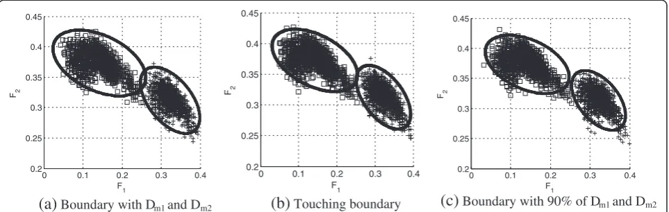
Ratnasingam and Collins [11] have suggested that the relative quality of the spectral information that can be obtained from feature spaces can be determined by using the clusters of responses from two reflectance spectra to determine decision boundaries for distinguishing bet-ween the two spectra and then determining the per-centage of feature points that fall within the correct boundary. The cluster of points in a two-dimensional feature space for two particular reflectance spectra shown Figure 5 is typical of the clusters of responses that have been obtained from many reflectance spectra. Since the typical cluster of points is not circular the distribution of points has been characterised using a Mahalanobis distance. For a multivariable normal distri-bution, the Mahalanobis distance between the centre of the distributionCand a pointPis defined as follows:

D2M ¼ðPCÞ 0_Σ1

PC

ð Þ; ð10Þ

whereΣis the covariance matrix of the distribution. The first step in determining the boundaries for a par-ticular pair of reflectances is to find the centre of each cluster of responses using the average position of all the responses in the cluster. The Mahalanobis distances (Dm1is

the Mahalanobis distance from cluster centre 1 andDm2is -20 0 20 40 60 80 100

0 2000 4000 6000 8000 10000 12000

Solar elevation (deg)

Correlated colour temperature (K)

Mean Correlated colour temperature Standard deviation

Figure 3The relationship between solar elevation and both the mean CCT and its standard deviation observed in data measured in Granada over a 2-year period under widely varying weather conditions.

400 450 500 550 600 650 700 60

70 80 90 100 110 120 130

Wavelength

Relative power

6500K CIE model

6440K (11.21 GMT, 04/12/1996) 6595K (16.36 GMT, 04/12/1996)

(7)

the Mahalanobis distance from cluster centre 2) that go through the midpoint (P) of the line connecting the two mean points (C1andC2) of the pairs of clusters were then

calculated.

D2m1¼ðPC1Þ0Σ11ðPC1Þ ð11Þ

D2m2¼ðPC2Þ0Σ21ðPC2Þ; ð12Þ

whereΣ1−1and Σ2−1 are the inverse covariance matrices of

the clusters 1 and 2, respectively. The boundaries obtained usingDm1andDm2as the distances from the relevant

clus-ter centre lead to overlap of some of the clusclus-ter boundaries (shown in Figure 5a). To find the boundaries that just touch each other (referred to as the touching boundaries), the points on a boundary at a Mahalanobis distance slightly smaller than Dm1 and Dm2 from the respective cluster

centres were then calculated for both pairs of reflectances. Previously, Ratnasingam and Collins [11] have determined the touching boundaries by gradually increasing the Mahalanobis distances between the boundaries and the centres until the boundaries touched (shown in Figure 5b). This process maximises the number of responses that are correctly classified; however, it is time consuming. To make the process of finding the Mahalanobis distance boundary simpler and to avoid any overlap, boundaries were drawn with the Mahalanobis distance of 90% of the distanceDm1andDm2(shown in Figure 5c). Results such

as the typical results shown in Figure 5 show that the boundaries drawn with 90% ofDm1andDm2do not

over-lap but will slightly underestimate the ability to correctly identify the source of a feature point generated using either the model-based or projection-based algorithms. Slightly underestimating the identification performance is

acceptable compared to overestimating the performance of an algorithm.

4.2. Selecting the boundary parameters based on the phase of a day

The possible benefits of employing the phase of the day in conjunction with date information when identifying the possible source of a set of features obtained using a pixel-level colour constancy algorithm have been assessed using the measured daylight spectra [20]. In particular, the daylight spectra measured in the year of 1996 (daylight spectra set 1) were used to determine the 90% ofDm1and Dm2boundaries for 100 pairs of reflectances. The daylight

spectra measured in the year of 1997 (daylight spectra set 2) was then used to generate the simulated sensor responses from which features were obtained. The per-centage of the feature points that fell within the correct boundary was then determined for each of the 100 pairs of reflectances in the test dataset.

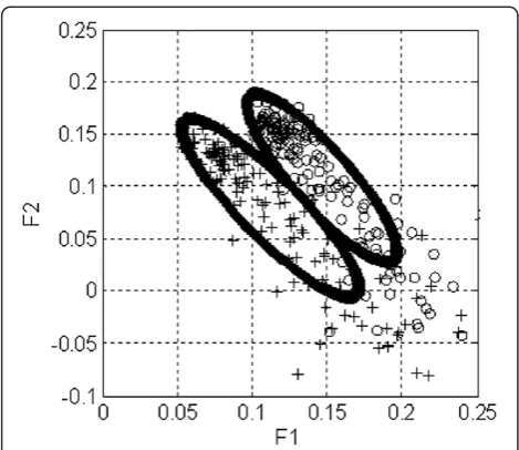
The features obtained from two Munsell reflectance samples (Munsell samples: 2.5R 9/2 and 5Y 7/1) that are separated by 6 units in CIELab space when illuminated by 146 daylight spectra (measured in the first day of every month in 1996) are shown in Figure 6. This figure also shows a Mahalanobis distance boundary around the different features obtained for each Munsell sample. Figure 7 shows the same Munsell pair (Munsell samples: 2.5R 9/2 and 5Y 7/1) projected on to the feature space when illuminated by daylight measured just after sunrise (solar elevation less than 20°), in the middle of the day (solar elevation greater than 20°) and just before sunset (solar elevation less than 20°). The respective Mahalanobis distance boundaries are also shown in Figure 7. By comparing Figures 6 and 7, it can be seen that

0 0.1 0.2 0.3 0.4

0.2 0.25 0.3 0.35 0.4 0.45

F 1

F2

0 0.1 0.2 0.3 0.4

0.2 0.25 0.3 0.35 0.4 0.45

F₁

F2

0 0.1 0.2 0.3 0.4

0.2 0.25 0.3 0.35 0.4 0.45

F 1

F2

(a)

Boundary with Dm1 and Dm2

(b)

Touching boundary

(c)

Boundary with 90% of Dm1 and Dm2

(8)

taking the phase of the day into account has made the cluster of features obtained from each Munsell colour smaller, particularly in the middle of the day (elevation larger than 20°). A small cluster size means that a larger number of perceptually similar reflectances could be iden-tified. This suggests that incorporating the phase of the day with quarter of the year (season) information into

account to determine the boundary settings in the feature space obtained from either the model-based or the projection-based algorithms could improve the ability to distinguish similar or very similar colours. However, close investigation of Figure 7 shows that in the spaces shown in Figure 7a,c the mean positions of the clusters have shifted to the lower right-hand side and the cluster size is relatively large compared to Figure 7b. The reason could be that at midday direct sunlight dominates and the vari-ation in CCT during midday is small (shown in Figure 3). The reason for the larger cluster sizes in the periods just after sunrise and just before sunset compared to the mid-dle of the day is the larger variations in CCT just after sunrise and just before sunset for smaller elevation of the Sun (shown in Figure 3). Comparing the typical ries shown in Figure 7a,c it can be seen that the bounda-ries of this typical pair do not appear to significantly be different between morning and evening. However, com-pared to using the same boundaries for morning and evening a significant performance improvement (22.8%) was obtained using two different boundaries for morning and evening.

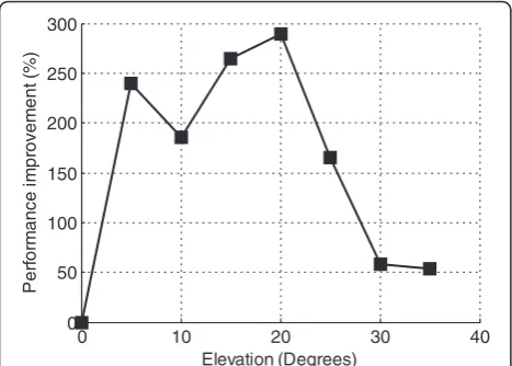
It is possible to switch the boundaries between just after sunrise, the middle of day and just before sunset at different threshold values for the solar elevation. To investigate the impact of the solar elevation threshold, when switching the boundary between different phases of day, we varied the elevation threshold and tested the performance of the proposed approach for recognition of perceptually similar colours. In particular, we varied the threshold between 0 and 35°. In this investigation, we used the 3-CIELab units Munsell test set and the mea-sured daylight spectra (set 1). The projection algorithm

Figure 6Typical feature space formed by the model-based algorithm when illuminating a pair of Munsell samples (Munsell samples: 2.5R 9/2 and 5Y 7/1) by daylight spectra measured between 5.00 and 20.00 GMT (daylight set 1).A Mahalanobis distance boundary is drawn for each Munsell sample (shown in thick solid black line). A cross and a small circle show the feature obtained using model-based algorithm by illuminating the Munsell samples: 2.5R 9/2 and 5Y 7/1 illuminated by one of the CIE standard illuminant, respectively.

0 0.05 0.1 0.15 0.2 0.25

-0.1 -0.05 0 0.05 0.1 0.15 0.2 0.25

F1

F2

0 0.05 0.1 0.15 0.2 0.25

-0.1 -0.05 0 0.05 0.1 0.15 0.2 0.25

F1

F2

0 0.05 0.1 0.15 0.2 0.25

-0.1 -0.05 0 0.05 0.1 0.15 0.2 0.25

F1

F2

(b)

Midday, Elevation>=20 Degrees

(a)

Morning, Elevation<20 Degrees

(c)

Evening, Elevation<20 Degrees

(9)

was used to extract features from the simulated noisy sen-sor responses to the pairs of reflectances in the Munsell test reflectance datasets when illuminating with measured daylight spectra. The Mahalanobis distance boundary was then determined for both members of each pair of Munsell colours. The percentage of points from the test data that fell inside the correct Mahalanobis distance boundary in the pair was then counted. This test was carried out on all the 100 pairs in a test reflectance set and the percentage of correctly classified points was calcu-lated. The results are shown in Figure 8. From these results it can be seen that switching the boundaries when the solar elevation is at 20° gives the best performance. Therefore, we used 20° as the threshold for solar elevation for switching the boundary settings in a day in the rest of the results presented in this article.

Another factor that affects the results obtained is the number of periods (with equal time length) in a year. To find the optimum number of periods in a year we varied the number of periods from 12 (each month starting from January) to 2 (every 6 months) without considering the seasons. These results are shown by filled square in Figure 9. When dividing the year into four we also divided the boundaries considering the months in the four seasons and the result is shown by star. From these results it can be seen that dividing the year into four equal periods by considering the seasonal information (here, quarter 1 consists of months 12, 1 and 2; quarter 2 consists of months 3, 4 and 5; quarter 3 consists of months 6, 7 and 8; quarter 4 consists of months 9, 10 and 11) results the best performance. This was done based on the seasonal information in Granada, Spain. It is therefore very unlikely that this same division of the year be the best method of grouping days elsewhere in

the world. However, our results suggest that it will be sensible to take into account information about regional annual weather patterns.

Based on the above investigation a solar elevation of 20° has been used to separate each day into three parts. In addition, days have been grouped into four quarters, in which quarter 1 consists of months 12, 1 and 2; quarter 2 consists of months 3, 4 and 5; quarter 3 consists of months 6, 7 and 8; quarter 4 consists of months 9, 10 and 11. In the rest of the article, we will use these four quarters to determine the boundary settings. A Mahalanobis dis-tance boundary for each pair of test reflecdis-tances was then obtained for each of these set of illuminants. Subse-quently, the phase of the day and the date that a measured daylight spectrum was obtained in the second year was used to determine the appropriate set of classification boundaries from the 12 available sets of boundaries. The impact of this method of adapting the Mahalanobis dis-tance boundaries was investigated with features obtained using both the model-based and projection-based algo-rithms (parameters listed in Tables 1 and 2).

4.3. Results for 30-dB SNR

The variability in the features extracted using pixel-level colour constancy algorithms depend upon both the CCT of the illuminant and the sensors SNR. To investigate the effect of different noise levels both the model-based and projection-based algorithms were used to obtain features from sensor responses with a 30-dB SNR. Figure 10 shows a typical reflectance sample projected onto the feature space when the SNR of both of the responses are 30 and 40 dB. It can be seen that when the noise level increases, the variation in the extracted features also increases. This must have an impact on the ability to distinguish between reflectances.

0 10 20 30 40

0 50 100 150 200 250 300

Elevation (Degrees)

P

e

rf

or

m

ance i

m

pr

ovem

ent

(

%

)

Figure 8Test results when varying the threshold of the solar elevation in the steps of 5° between 0 and 35°.In this figure, y-axis shows the performance improvement of the projection-based algorithm obtained by incorporating the auxiliary information (solar elevation, phase of day and time of year).

2 4 6 8 10 12

30 32 34 36 38 40 42

Number of periods in a year

Average recognition (%)

(10)

Table 3 shows the performance of the model-based and projection-based algorithms when the SNR of the sensor responses is 30 dB. The results obtained from the features extracted with the two algorithms have been comparable and it has been found that using phase of the day and quar-ter of year information improves the results obtained in most of the cases. However, the most important conclusion from these results and the results shown in Table 4 confirm that as expected the larger variability of the extracted features caused by the increase in the amount of noise in the data degrades the quality of information that can be obtained from the features. Even when the phase of the day

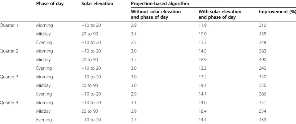
and date information is used it is therefore important to ensure that the SNR of the sensor responses is as high as possible. We also applied our proposed approach on the original Finlayson and Drew’s [10] algorithm and the test results are given in Table 5. Comparing the column 4 of Tables 3 and 5 it can be seen that our modified algorithm (projection-based algorithm) gives significantly better per-formance compared to that of the original Finlayson and Drew’s [10] algorithm. Moreover, applying our proposed approach of utilising the auxiliary information (phase of day, time of year and solar elevation) results in significant improvement (see column 6 of Table 5).

-0.6 -0.5 -0.4 -0.3 0

0.05 0.1 0.15 0.2 0.25 0.3 0.35 0.4

F1

F2

-0.6 -0.5 -0.4 -0.3

0 0.05 0.1 0.15 0.2 0.25 0.3 0.35 0.4

F1

F2

(a)

40dB SNR

_(b)

_{30dB SNR}

Figure 10A typical Munsell reflectance projected on the feature space when illuminated with 20 spectra of daylight with sensor noise of (a) 40 dB and (b) 30 dB.Each star shows the feature obtained with Munsell sample 2.5R 9/2 and the CIE standard daylight illuminant with CCT 6,500 K.

Table 3 Performance of the model-based and projection-based algorithms when applying the sensor responses generated by 80-nm FWHM evenly spread sensors

Phase of day Solar elevation

Projection-based algorithm Model-based algorithm

Without solar elevation and phase of day

With solar elevation and phase of day

Improvement (%) Without solar elevation and phase of data

Improvement (%)

Quarter 1 Morning ₋10 to 20 13.9 12.4 ₋10.7 13.9 11.8 ₋15.1

Midday 20 to 90 17.4 20.0 +14.9 17.1 20.1 +17.5

Evening ₋10 to 20 12.0 11.9 ₋0.8 12.2 11.9 ₋2.4

Quarter 2 Morning ₋10 to 20 15.3 15.5 +1.3 15.5 15.8 +1.9

Midday 20 to 90 16.2 20.1 +24.1 16.0 20.4 +27.5

Evening −10 to 20 14.2 14.0 −1.4 13.9 14.0 +0.7

Quarter 3 Morning −10 to 20 13.8 14.1 +2.2 13.5 14.0 +3.7

Midday 20 to 90 15.8 20.1 +27.2 15.7 20.4 +29.9

Evening −10 to 20 14.3 15.0 +4.9 14.0 15.1 +7.8

Midday 20 to 90 15.0 19.4 +29.3 14.8 19.5 +31.8

Evening −10 to 20 13.4 15.1 +12.7 13.3 15.3 +15.0

(11)

4.4. Results for 40-dB SNR

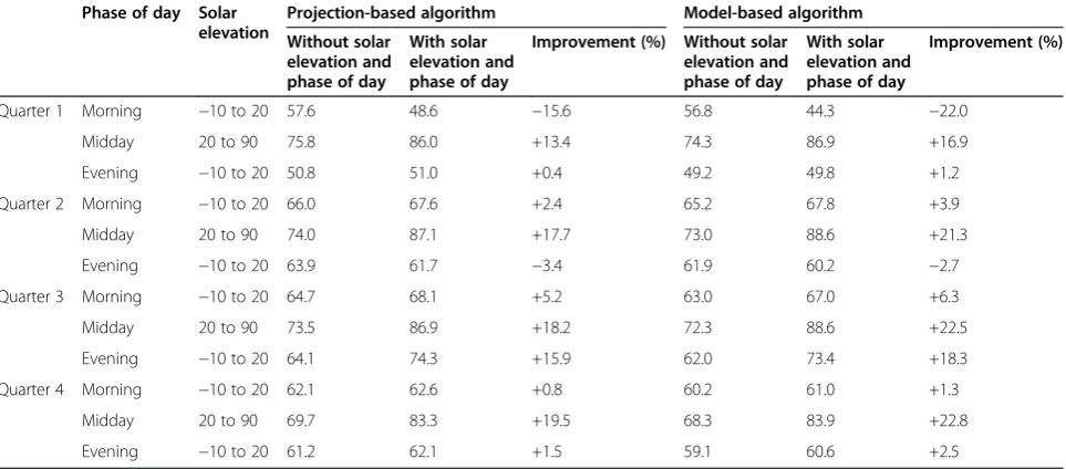
The results obtained from the test Munsell test data for 40-dB SNR are given in Tables 4, 6 and 7. The first conclusion from Tables 4, 6 and 7 is that the results obtained using features extracted with the model-based and projection-based algorithms are almost identical. The second conclusion is that the percentage perfor-mance improvement obtained when using the solar elevation and phase of day information to determine the

appropriate decision boundaries show that this ancillary information is helpful and has improved the performance in most of the cases. In particular, using this ancillary information reduces the quality of the results obtained in only 14 of the 72 comparisons in these tables. All of these 14 cases occur, just after sunrise (morning) and just before sunset (evening) when, as shown in Figure 3, significant variations in CCT at smaller solar elevations occur. Since the decision boundaries that are created without using Table 4 Test results of the model-based and projection-based algorithms when applying the sensor responses

generated by 80-nm FWHM evenly spread sensors Phase of day Solar

elevation

Improvement (%) Without solar elevation and phase of day

Improvement (%)

Quarter 1 morning −10 to 20 35.2 23.6 −32.9 34.6 19.6 −43.3

midday 20 to 90 41.4 57.2 +38.2 37.8 57.6 +52.4

evening −10 to 20 27.5 25.4 −7.6 26.7 24.5 −8.2

Quarter 2 Morning −10 to 20 39.1 38.8 −0.8 38.5 39.5 +2.6

midday 20 to 90 36.7 57.7 +57.2 34.1 58.5 +71.5

evening −10 to 20 28.6 35.8 +25.2 26.3 35.5 +34.9

midday 20 to 90 35.6 56.6 +59.0 32.5 57.7 +77.5

evening −10 to 20 32.0 44.6 +39.4 28.8 43.6 +51.4

midday 20 to 90 30.2 51.2 +69.5 27.4 51.4 +87.6

evening −10 to 20 27.5 33.8 +22.9 24.8 32.6 +31.4

In this test, Munsell samples separated by 3-CIELab units and measured daylight spectra were applied. Each sensor response was multiplied by normally distributed hundred random numbers with a mean value of 1 and standard deviation 1% and the resulting linear responses were quantised to 10 bits. The Mahalanobis distance boundary settings were applied in three phases of the day (morning, midday and evening) with elevation threshold of 20°.

Table 5 Performance of the original Finlayson and Drew’s [10] algorithm when applying the sensor responses generated by 80-nm FWHM evenly spread sensors

Phase of day Solar elevation Projection-based algorithm

Improvement (%)

Quarter 1 Morning ₋10 to 20 2.9 11.9 310

Midday 20 to 90 3.4 19.0 458

Evening ₋10 to 20 2.5 11.2 348

Quarter 2 Morning ₋10 to 20 3.0 14.5 383

Midday 20 to 90 3.2 18.9 490

Evening −10 to 20 3.0 13.2 340

Quarter 3 Morning −10 to 20 3.0 13.2 340

Midday 20 to 90 3.0 19.1 536

Evening −10 to 20 2.9 14.1 386

Quarter 4 Morning −10 to 20 3.1 14.0 351

Midday 20 to 90 2.9 18.4 534

Evening −10 to 20 2.7 14.4 433

(12)

ancillary information cover a larger area of the feature space this consequence of using the ancillary information is not surprising. More importantly, the results in Tables 4, 6 and 7 show that the suggested method of using ancillary information always improves our ability to distinguish between perceptually similar reflectances during the mid-dle period of each day. This combined with the fact that the improvements in some cases are as large as 300%

suggests that using ancillary information will significantly improve the ability to draw correct conclusions from the features from pixel-level colour constancy algorithms. Finally, comparing the results in Tables 4, 6 and 7 suggests that these improvements will particularly be most signifi-cant when distinguishing between objects whose reflec-tance spectra are so similar that an expert would find them impossible to distinguish.

Table 6 Test results of the model-based and projection-based algorithms when applying the sensor responses generated by 80-nm FWHM evenly spread sensors

Improvement (%)

Quarter 1 Morning −10 to 20 13.5 10.8 −20.0 12.5 8.2 −34.4

Midday 20 to 90 11.6 26.4 +128 9.3 25.8 +177

Evening −10 to 20 9.0 8.2 −8.9 8.2 7.3 −10.9

Quarter 2 Morning −10 to 20 13.8 13.3 −3.6 12.7 12.9 +1.6

Midday 20 to 90 9.0 26.5 +194 7.5 26.6 +255

Evening −10 to 20 7.6 13.4 +76.3 6.1 13.0 +113

Midday 20 to 90 8.9 26.1 +193 7.2 26.1 +263

Evening −10 to 20 9.8 13.3 +35.7 7.6 11.5 +51.3

Midday 20 to 90 7.2 23.4 +225 5.8 23.2 +300

Evening −10 to 20 7.1 9.0 +26.8 5.6 7.9 +41.0

In this test, Munsell samples separated by 1-CIELab units and measured daylight spectra were applied. Each sensor response was multiplied by normally distributed hundred random numbers with a mean value of 1 and standard deviation 1% and the resulting linear responses were quantised to 10 bits. The Mahalanobis distance boundary settings were applied in three phases of the day (morning, midday and evening) with elevation threshold of 20°.

Table 7 Performance of the model-based and projection-based algorithms when applying the sensor responses generated by 80-nm FWHM evenly spread sensors

Improvement (%)

Quarter 1 Morning ₋10 to 20 57.6 48.6 ₋15.6 56.8 44.3 ₋22.0

Midday 20 to 90 75.8 86.0 +13.4 74.3 86.9 +16.9

Evening ₋10 to 20 50.8 51.0 +0.4 49.2 49.8 +1.2

Quarter 2 Morning ₋10 to 20 66.0 67.6 +2.4 65.2 67.8 +3.9

Midday 20 to 90 74.0 87.1 +17.7 73.0 88.6 +21.3

Evening −10 to 20 63.9 61.7 −3.4 61.9 60.2 −2.7

Midday 20 to 90 73.5 86.9 +18.2 72.3 88.6 +22.5

Evening −10 to 20 64.1 74.3 +15.9 62.0 73.4 +18.3

Midday 20 to 90 69.7 83.3 +19.5 68.3 83.9 +22.8

Evening −10 to 20 61.2 62.1 +1.5 59.1 60.6 +2.5

(13)

5. Conclusions

If the spectrum of the scene illuminant can be approxi-mated by the spectrum of a blackbody then pixel-based colour constancy algorithms can be used to extract features that are almost independent of the illuminant. The blackbody approximation used to derive these algo-rithms is most appropriate when the illuminant is daylight. Results have been presented using measured daylight spectra that show that the residual illuminant dependence of the features is caused by a combination of noise, finite spectral width and the non-blackbody spectrum. The latter effect means that the features ob-tained from a reflective surface vary with the spectrum of the daylight, usually characterised by its CCT. An inves-tigation of the CCTs of daylight spectra measured in Granada, Spain, over 2 years shows that the CCT of day-light varies with the solar elevation and to a lesser extent on the date. We investigated the optimum number of periods in a year and the solar elevation threshold that results the best performance. Based upon these observa-tions, the measured daylight spectra for 1 year have been used to create 12 sets of illuminants. These illuminants have then been used to create boundaries in the feature space that can be used to distinguish between pairs of sur-faces whose colours are very good matches to each other. Using the data from a second year which is different from the training set, it has been shown that for good quality images the ability to successfully distinguish these surfaces is significantly improved on average using the phase of the day and date information by 33.7 and 45.4% for projection-based and model-based algorithms, respec-tively. In particular, a larger improvement (average im-provement: 85.9 and 113.7%) was obtained during the middle period of each day which is defined as when the solar elevation is larger than 20°. This method would therefore seem to be particularly useful for scenes illumi-nated by daylight in the middle of the day. One possible application that suits these restrictions is precision far-ming, in which machine vision techniques can be used to target the treatment of small areas of a field or individual plants [22,23]. In the future, the possibility of optimising the sensor characteristic and using a third illuminant invariant feature will be investigated.

Competing interests

The authors declare that they have no competing interests.

Acknowledgement

This study was done while Sivalogeswaran Ratnasingam was at the University of Oxford, Oxford, UK. Javier Hernández-Andrés's work was supported by the Ministry of Economy and Competitiveness, Spain, under research grant DPI2011-23202.

Author details

1_{Department of Engineering Science, University of Oxford, OX1 3PJ Oxford,}

UK.2Department of Optics, Sciences Faculty, University of Granada, Granada 18071, Spain.3_{The Australian National University, Canberra ACT 0200,}

Australia.4_{NICTA Canberra Research Laboratory, 7 London Circuit, Canberra} ACT 2601, Australia.

Received: 5 August 2012 Accepted: 16 February 2013 Published: 18 March 2013

References

1. SD Buluswar, BA Draper, Color machine vision for autonomous vehicles. Eng. Appl. Artif. Intell.11, 245–256 (1998)

2. S Hordley, Scene illuminant estimation: past, present, and future. Color Res. Appl.31(4), 303–314 (2006)

3. DH Foster, Color constancy. Visi. Res.51(7), 674–700 (2011). doi:10.1016/j. visres.2010.09.006

4. B Funt, K Barnard, L Martin, Is colour constancy good enough? inProceeding ECCV '98 Proceedings of the 5th European Conference on Computer Vision-Volume I - Vision-Volume I(Springer-Verlag, London, UK, 1998), pp. 445–459. ISBN 3-540-64569-1

5. J Romero, J Hernández-Andrés, JL Nieves, JA García, Color coordinates of objects with daylight changes. Color Res. Appl.28, 25–35 (2003) 6. M Ebner,Color Constancy(Wiley-IS&T Series in Imaging Science and

Technology, New York, 2007)

7. JA Marchant, CM Onyango, Shadow-invariant classification for scenes illuminated by daylight. J. Opt. Soc. Am. A17, 1952–1961 (2000) 8. GD Finlayson, SD Hordley, Color constancy at a pixel. J. Opt. Soc. Am. A

18, 253–264 (2001)

9. J Romero, J Hernández-Andrés, JL Nieves, EM Valero, Spectral sensitivity of sensors for a color-image descriptor invariant to changes in daylight conditions. Color Res. Appl.31(5), 391–398 (2006)

10. GD Finlayson, MS Drew, 4-sensor camera calibration for image

representation invariant to shading, shadows, lighting, and specularities, in ICCV 2001: International Conference on Computer Vision, Volume 2(IEEE, Los Alamitos, 2001), pp. 473–480

11. S Ratnasingam, S Collins, Study of the photodetector characteristics of a camera for color constancy in natural scenes. J. Opt. Soc. Am. A27, 286–294 (2010) 12. S Ratnasingam, S Collins, J Hernández-Andrés, Optimum sensors for color

constancy in scenes illuminated by daylight. J. Opt. Soc. Am. A27, 2198–2207 (2010)

13. D Forsyth, J Ponce,Computer Vision: A Modern Approach(Prentice-Hall, Upper Saddle River, NJ, 2003)

14. The Munsell Color Science Laboratory. http://www.cis.rit.edu/mcsl/online/cie.php 15. Database– “Munsell Colours Matt”. ftp://ftp.cs.joensuu.fi/pub/color/spectra/

mspec/

16. A Abrardo, V Cappellini, M Cappellini, A Mecocci, A Abrardo, V Cappellini, M Cappellini, A Mecocci, Art-works colour calibration using the VASARI scanner, inPublished in Fourth Color Imaging Conference: Color Science, Systems, and Applications(, Scottsdale, Arizona, 1996), pp. 94–96. ISBN 0-89208-196-1

17. JY Hardeberg,Acquisition and reproduction of color images: colorimetric and multispectral approaches, Ph.D. dissertation, Ecole Nationale Supérieure des Télécommunications, 1999

18. M Mahy, L van Eycken, A Oosterlinck, Evaluation of uniform color spaces developed after the adoption of CIELAB and CIELUV. Color Res. Appl.19(2), 105–121 (1994)

19. HC Lee,Introduction to Color Imaging Science(Cambridge University Press, Cambridge, MA, 2005), pp. 46–47. 138–141 and 450–459

20. J Hernández-Andrés, J Romero, JL Nieves, RL Lee Jr, Color and spectral analysis of daylight in southern Europe. J. Opt. Soc. Am. A18, 1325–1335 (2001) 21. S Kalogirou,Solar Energy Engineering: Processes and Systems(Academic Press,

New York, 2009)

22. SR Herwitz, LF Johnson, SE Dunagan, RG Higgins, DV Sullivan, J Zheng, BM Lobitz, JA Brass, Imaging from an unmanned aerial vehicle: agricultural surveillance and decision support. Comput. Electron. Agric.44(1), 49–61 (2004) 23. MS Moran, Y Inoue, EM Barnes, Opportunities and limitations for

image-based remote sensing in precision crop management. Remote Sens. Environ.61(3), 319–346 (1997)

doi:10.1186/1687-5281-2013-14

Cite this article as:Ratnasingamet al.:Analysis of colour constancy

algorithms using the knowledge of variation of correlated colour

temperature of daylight with solar elevation.EURASIP Journal on Image