Article
1
Spatial Dependence Modeling of Wind Resource under
2
Uncertainty Using C-Vine Copulas and Its Impact on
3
Solar-Wind Energy Co-Generation
4
Apurva Narayan 1, *, Kumaraswamy Ponnambalam 1 and Sheree A. Pagsuyoin2
5
1 University of Waterloo, Ontario, Canada N2L 3G1; {a22naray, ponnu}@uwaterloo.ca
6
2 University of Massachusetts Lowell, Massachusetts, USA 01854; [email protected]
7
* Correspondence: [email protected], Tel.: +1-519-888-4567 x31450 8
Abstract: Investments in wind and solar power are driven by the aim to maximize the utilization of
9
renewable energy (RE). This results in an increased concentration of wind farms at locations with higher
10
average wind speeds and of solar panel installations at sites with higher average solar insolation. This is
11
unfavourable for energy suppliers and for the overall economy when large power output fluctuations occur.
12
Thus, when evaluating investment options for spatially distributed RE systems, it is necessary to model
13
resource fluctuations and power output correlations between locations. In this paper, we propose a
14
methodology for analyzing the spatial dependence, accurate modeling, and forecasting of wind power
15
systems with special consideration to spatial dispersion of installation sites. We combine vine-copulas with
16
the Kumaraswamy distribution to improve accuracy in forecasting wind power from spatially dispersed
17
wind turbines and to model solar power generated at each location. We then integrate these methods to
18
formulate an optimization model for allocating wind turbines and solar panels spatially, with an end goal
19
of maximizing overall power generation while minimizing the variability in power output. A case study of
20
wind and solar power systems in Central Ontario, Canada is also presented.
21
Keywords: renewable energy; wind and solar power; Kumaraswamy distribution; C-Vine copula
22 23
1. Introduction
24
Wind power is one of the world’s largest and most accessible high intensity renewable energy resource,
25
with solar power fast becoming a widely implemented renewable resource [1]. Globally, there are
26
increasing efforts to tap more into these renewable energy sources; however, their intermittent availability
27
presents one barrier for the renewable energy-based systems to entirely meet energy demands [2]. Wind
28
fluctuations can be abrupt and significant, causing problems with the ability to generate steady energy
29
outputs. Also, due to the stochastic nature of wind, it is difficult to accurately forecast wind power
30
generation by considering only temporal wind behavior when other factors such as wind farm topology and
31
turbine characteristics are equally important [3]. On the other hand, while the availability of solar energy is
32
relatively constant, solar power output exhibits high sensitivity to slight changes in solar insolation [4].
33 34
Another challenge associated with renewable energy systems is their integration into the main power
35
grid. Renewable energy installations can be geographically sparsely distributed despite being part of the
36
same power grid, leading to sub-optimal power transactions within the grid [5]. Decisions on where to place
37
these installations are often based on the availability of wind and solar resources in order to maximize
38
perceived power outputs [6]. This leads to localized concentrations of installations in areas of high wind or
39
solar availability, which can become highly unfavourable for energy suppliers due to increased power
40
fluctuations and overall system instability [6].
41 42
Previous researchers have examined the possibility of smoothing fluctuations in wind power
43
generation through employing geographically dispersed systems, or by interconnecting existing dispersed
44
systems [7, 8]. For example, system reliability has been found to increase with turbine size in wind farms
45
[9], while interconnection has been shown to greatly impact the reliability and stability of renewable energy
46
systems [10].
47 48
In this paper, we propose a methodology for analyzing the spatial dependence, accurate modeling, and
49
forecasting of wind power generation with special consideration to temporal variations in power output and
50
spatial dispersion of installation sites. The rest of this paper is organized as follows: Section 2 provides a
51
brief review of literature related to wind and solar power systems modeling. Section 3 introduces the three
52
mathematical concepts that serve as the foundations of our proposed methodology: the Kumaraswamy
53
distribution, the theory of copulas, and vine-copulas. Section 4 discusses our proposed model for the
54
optimal allocation of renewable energy generation technologies while Section 5 presents a case application
55
of the proposed methodology. Finally, Section 6 summarizes the findings and intellectual contributions of
56
this study.
57
2. Literature Review
58
Linear correlation coefficients provide general information about the interdependence of wind power
59
generated at spatially distributed sites [11]; however, they do not uniquely describe the structure of this
60
dependence [11]. Further, they do not provide actionable information that is helpful to system planners and
61
operators. For example, linear correlation coefficients are not useful in determining the duration in a year
62
when the aggregate wind power in a system will be above or below a specified threshold value even when
63
coupled with data on the marginal distributions of wind power at each installation, as dependence relations
64
are nonlinear. A potential method for mathematically describing the dependency structure among wind
65
power systems involves using joint distribution functions [12]. However, multivariate distribution models
66
are currently not available for such systems, and common joint distributions do not accurately fit wind
67
power data [12]. A possible workaround suggested by Kroese et al [13] involves decomposing the assumed
68
correlation matrix using Cholesky decomposition, but this is only applicable if random variables are linearly
69
correlated.
70 71
It has been demonstrated that wind speeds are characterized by normal distributions and
non-72
linear dependence [6]. This becomes problematic in multivariate analysis; when multivariate data are not
73
normally distributed, accurate quantiles of the sums of margins cannot be calculated from the sums of
74
variances and covariances which makes modeling these random variables (wind speeds in our case) more
75
challenging.
77
Goethe and Schnieders [6] modeled the univariate time series of wind speed at several wind farms in
78
Germany using a seasonal autoregressive moving average (ARMA) model proposed by Benth and Benth
79
[14]. To model the correlation between multiple wind farm locations, they analyzed the correlation between
80
the residuals of the various univariate time series and fit copulas to the residuals, thus developing
copula-81
GARCH (generalized autoregressive conditional heteroskedasticity) models.
82 83
A more appropriate approach for modeling non-linear, non-normal and more complex dependency
84
structure in data is by directly using appropriate copulas [6, 15-18]. Copulas are applied widely in finance
85
[19, 20], and they possess unique characteristics that make them highly attractive in modeling wind power
86
[18]. Of these characteristics, the most important is the ability of copulas to model the dependence structure
87
of data independent of the marginal distributions of the participating variables. This feature is very critical
88
because wind power outputs at different locations are often significant at the grid nodes they are infused
89
and modeling them using single marginal distribution is not possible. Therefore, finding this dependence
90
in power outputs independent of marginal distributions is of great advantage for system planners as it allows
91
modeling wind power generation more accurately.
92 93
The correlations among wind power generated at different locations are usually estimated from
94
parameters such as separation distance and averaging period, among others [21, 22, 23]. If only basic
95
information is available about the locations of wind turbines, an accurate model of the dependency structure
96
of wind power generated at these locations can be produced using copulas. Consequently, the selection of
97
an appropriate copula function is very important, as inappropriate selection can lead to unacceptable errors.
98
Of all copulas, the Gaussian copula is the most commonly used copula due to its computational
99
convenience; however, its suitability in wind power analysis has not been rigorously investigated. The
100
standard Gaussian copula has been previously used to model wind power in Europe based on a qualitative
101
assessment of Q-Q plots [17]. Louie (2012) adopted a more comprehensive approach by first testing a
102
number of standard copulas on wind speed data, and then eventually selecting Archimedean copulas [23].
103 104
In modeling wind power, copulas have the highest utility in forecasting and in generating scenarios for
105
optimization simulations [19]. These scenarios are necessary in stochastic programming, which is a critical
106
decision tool in power systems analysis and planning research. For example, Gaussian copulas have been
107
used to evaluate short-term scenarios for wind power generation [24], while empirical copulas have been
108
used in modeling the dependency structure between the wind speed and the wind power output [25]. A
109
quantile-copula kernel density estimator has also been used to improve probabilistic wind power forecasts
110
[26].
111 112
With respect to solar energy, temporal modeling of solar power generation has been done using
113
generalized distribution functions that were subsequently optimized to ensure reliable and higher power
114
outputs [27]. Solar irradiation is most often modeled using the Hollands and Huggets distribution, which
115
can be approximated by the Gamma distribution [28]. To our knowledge, there has been no attempt to date
to model solar power generation using other types of probability distributions. Similar to wind power
117
generation, the dependence structure of solar systems is usually quantified by measures of association such
118
as linear correlation coefficients [29]. But in contrast to wind power generation, the spatial variability in
119
solar power generation in reasonably sized grids is not significant; thus modeling the spatial dependence of
120
solar power generated between dispersed locations is not necessary [30] but can be done with the method
121
we propose for wind power.
122
3. Methodology
123
Wind speed patterns and their spatial dependencies are generally non-Gaussian and non-linearly 124
correlated [14]. Since system planners are more interested in modeling wind power generation than wind 125
speeds, this presents a challenge because there is no standardization in modeling wind power using a 126
specific probability distribution. Therefore, in the present study, we use the Kumaraswamy distribution 127
for the temporal modeling of wind power generated at each site, and applied the concept of vine-copulas 128
to model wind power dependencies. 129
3.1 Kumarawamy Distribution
130
First introduced in 1980, the double bounded Kumaraswamy distribution is a continuous probability 131
distribution that was originally developed for hydrology applications [26]. It is equivalent to the Beta 132
distribution but has a simpler analytical formulation, making it more efficient in computational 133
simulations. More importantly for this study, the Kumaraswamy distribution is selected because (i) 134
renewable power is a non-linear transformation of its resource (ex. wind power from wind speed) and (ii) 135
its simple analytical form allows for its easy integration with copulas. 136
137
The probability density function (PDF, ( ( )) and cumulative density function (CDF, ( ( )) 138
formulations of the Kumaraswamy distribution are given in Eq. 3.1 and Eq. 3.2, respectively, where a and 139
b are shape parameters describing the distribution. 140
141
( ) = (1 − ) (3.1)
Where, 142
> 0, > 0and [0,1] (3.2)
143
It has many of the same properties as the Beta distribution but has some advantages in terms of
144
tractability. The Kumaraswamy densities have similar behavior as the Beta densities such as they are
145
unimodal, uniantimodal, increasing, decreasing or constant depending on the parameters. Therefore, based
146
on the values of the shape parameters the densities take specific shape and exhibit certain properties such
147
as, if a > 1 and b > 1 then the density is unimodal, if a > 1 and b ≤ 1 then the density is increasing, a < 1and
148
b < 1 then the density is uni-antimodal, and a ≤ 1 and b > 1 then the density is decreasing. The densities are
149
log-concave if and only if the shape parameters are greater than or equal to 1.
In addition to hydrology, Kumaraswamy distribution is now widely used including in
151
finance, statistical design centering of integrated systems, among others [31, 32] .
152
3.2 Methodology
153
3.2.1 Copulas and the Sklar Theorem
154
Copulas were first introduced in 1959 by the mathematician Abe Sklar [33] and have since become
155
popular in describing the dependencies between random variables. Copulas are mathematical functions that
156
allow us to combine univariate distributions to obtain a joint distribution with a particular dependence
157
structure. The utility of a copula is most easily demonstrated in the use of distributions in probabilistic
158
analysis. To illustrate, recall that the CDF of a distribution is used to draw a random variate. Most commonly,
159
to draw a random value from a distribution, one starts by sampling from a uniform distribution, (0,1).
160
This sample is treated as an observation of the variable`s CDF; a sample can be drawn from the PDF by
161
generating a uniform random number and transforming it using the CDF to a random value.
162 163
Sklar’s theorem is the theoretical foundation of copulas. It states that for a given joint multivariate
164
distribution function and relevant marginal distributions for the corresponding random variables, there
165
always exists a copula function that relates the marginal distributions of the variables. Mathematically, this
166
can be derived as follows.
167 168
Let Fxybe a joint distribution with margins Fx and Fy.;then there exists a copula : [0,1] → [0,1] such
169
that
170
( ) = (1 − )
3.3
171
If the random variables, X and Y are continuous, then copula, C is unique; otherwise, C is uniquely
172
determined on the (range of X) × (range of Y).
173 174
Conversely if C is a copula and Fx and Fy are distribution functions, then the function Fxy is a joint 175
distribution with margins Fx and Fy. 176
C must be a function of particular type with certain properties as described by [33] and explained
177
further in [19].
178 179
The copula is further defined as follows. 180
C is a copula if : [0,1] → [0,1] and
181
(0, ) = ( , 0) = 0
182
(1, ) = ( , 1) =
183
( , ) − ( , ) − ( , ) + ( , ) ≥ 0 for all < , <
184
If C is differentiable once in its first argument and once in its second then, C is equivalent to
185
≥ 0 for all < , <
where um, vm, umi, vmi are marginal distribution functions.
187
This definition of a copula simply states that a copula is itself a distribution function, defined on
188
[0,1]2 with a uniform marginal. Each of the marginal distributions produces a probability of
one-189
dimensional events. The copula function takes these probabilities and maps them to a joint probability,
190
enforcing a relationship on the probabilities. Therefore, using copulas to build multivariate distributions is
191
a very flexible and powerful technique as it separates choice of dependence from the choice of marginal
192
[19].
193
Sklar’s theorem establishes one of the easiest ways of constructing copulas. In this case, if Fx and Fy
194
are the marginal distributions, then a copula is given by the formulation in Eq. 3.4.
195
( , ) = ( ( ), ( ))
3.4
3.2.2 Selection of the Appropriate Copula
196
A critical step in modeling data using copulas is the selection of the appropriate copula function from
197
among the family of copulas that best describes the given data set. The selection process is often based on
198
the analytical tractability of the copula function [34]. Three types of copulas are considered in this study:
199
Gumbel, Joe-Frank, and the Student t. The Gumbel copula is most suited for extreme distributions while
200
the Joe-Frank and Student t copulas are more suited for applications with heavy dependence on tails [19,
201
35].
202
The Gumbel copula is a bivariate Archimedean copula. It is an asymmetric copula that exhibits greater
203
dependence on the positive tail than on the negative tail. This copula is given by Eq. 3.5, where is the
204
parameter controlling the dependence between the marginal distributions and .
205
( , ) = exp (−[(− log ) + (− log ) ] ⁄ ) 3.5
The Joe-Frank copula, sometimes called the BB8 copula, is a two-parameter copula also from the
206
Archimedean family of copulas. The copula CDF is given by Eq. 3.6, where the parameter illustrates
207
the degree of dependence between the marginal distributions and , and the parameter is the degree
208
of freedom.
209
, ( , ) = 1 − 1 − 1 − (1 − ) 1 − (1 − ) ⁄ 3.6
where
210
≥ 1 0 ≤ ≤ 1
211
= 1 − (1 − ) and 0 ≤ , ≤ 1
212 213
The Student t copula allows for joint fat tails and an increased probability of joint extreme events
214
compared with the other copulas. Increasing the value of decreases the tendency to exhibit extreme
co-215
movements. The copula formulation is expressed in Eq. 3.7, where and are the parameters of the
216
copula, and is the inverse of the standard univariate t-copula with degrees of freedom, expectation
217
0 and variance [35]. The variables s and t are the random vectors obtained from the two marginal
218
distributions.
219
, ( , ) =
1
2 (1 − ) /
( ) ( )
1 + − 2 +
(1 − )
( )⁄
220
3.2.3 C-Vine Copulas
221
Joe [35] presented the first construction of a multivariate copula using (conditional) bivariate copulas,
222
while Bedford and Cooke [36] developed a more general construction method of multivariate densities and
223
introduced regular vines to organize different pair-copula constructions (PCCs). Vines are a graphical
224
representation of constraints in high dimensional probability distributions. They are used to specify
so-225
called PCCs, as introduced by Aas et al. [37].
226 227
Conventionally, a copula model is limited to a 1-parameter or 2-parameter specification of the
228
dependence structure, which represents a potentially severe empirical constraint. Clearly, when modeling
229
the joint distribution of multiple variables, such limited parameter models are unlikely to adequately capture
230
the dependence structure between variables. For example, the Gaussian copula lacks tail dependence.
231
Similarly, while the multivariate Student t copula is able to generate different tail dependence for each pair
232
of variables, it imposes the same upper and lower tail dependence across all pairs. These limitations are
233
overcome by the canonical vine (C-vine) model by building bivariate copulas of conditional distributions.
234
C-vine copulas are flexible multivariate copulas that are generated via hierarchical construction and can be
235
decomposed into a cascade of bivariate copulas. The basic principle is to model dependence using simple
236
local building blocks (pair-copulas).
237
4. Spatial and Temporal Modeling of Renewable Energy Resources
238
4.1 Algorithm for Temporal Modeling of Wind Power and for Scenario Generation
239
This section discusses the procedure for modeling wind power generation in various spatially
240
dispersed sites using the generalized Kumaraswamy distribution and C-Vine copulas.
241 242
Firstly, given temporal data sets (daily and seasonal) on the wind power generated at different
243
installations, we use the Kumaraswamy model to describe the probability distribution of each data set. We
244
obtain the model parameters for each hour of the day and for three seasons in the year lets call them Season
245
1, Season 2, and Season 3 using the Maximum Likelihood Estimate (MLE) method for distribution fitting
246
with historical data. This ensures that both hourly and seasonal variations are embodied in the distribution
247
models. Therefore, we create for each hour of the day within each of the three seasons a distribution from
248
all the measurements at that hour of day for all days within that season across a number of year. This leads
249
us to create 3 (season) × 24 (hours) = 72 distributions for each location. These distributions are then used
250
to choose a C-Vine model for the installation site under consideration.
251 252
In order to develop the C-Vine tree, one location must first be selected as the root node of the tree and
253
the others its children (nodes). This is accomplished by generating the Kendall rank correlation matrix, and
254
summing the correlations across each location with respect to the other locations. The location with the
255
maximum value of the Kendall rank correlation is chosen as the root node.
257
Once the C-vine tree is constructed, various families of bivariate copulas are then fitted to model the
258
dependence between the root node and each one of its children. We again use the MLE method to fit the
259
copulas, and use AIC/BIC (Akaike Information Criterion/ Bayesian Information Criteria) to evaluate the
260
goodness of fit. In this, pair-copula construction approach, a bivariate copula is fitted to the root node and
261
the child. Finally, we utilize the PCC-based tree to produce scenarios by drawing data from the PCC
262
followed by Kumaraswamy distribution for each hour of the day or season.
263
.
264
The algorithm for modeling of wind power is summarized in Table 1.
265
Step Specific Action
1 Fit Kumaraswamy distribution to each location’s hourly data for the three seasons (Season 1, Season 2 and Season 3) and obtain parameters for the distribution. 2 Compute the Kendall rank correlation matrix with correlation values where
Correlation Values, location with respect to location
3 Formulate the Vine tree, where root is the location with max(∑,: ).
4 Compute the Pair Copula Construction using the various copula options available 5 Generate scenarios from the PCC followed by inverse of Kumaraswamy CDF.
266
For scenario simulations using C-Vine, we generate the Vine matrix that defines the connections and
267
parameter matrices containing the parameters of each of the copulas defined by each link.
268
4.2 Algorithm for Spatial Modeling of Solar Power Generation 269
Similar to the procedure outlined in Section 4.1, we also use PCC for the spatial modeling of solar
270
power generation. Our goal here is to develop a standardized approach for spatial modeling of renewable
271
power sources. The procedure consists of two steps, as indicated in Table 2. Firstly, given the hourly (power
272
generation) data at each location for the three seasons (Season 1, Season 2, and Season 3), we use the
273
Kumaraswamy distribution to model hourly solar power outputs. We then generate scenarios by drawing
274
random variables from the Kumaraswamy CDF for each day for the three seasons. Although, solar power
275
is given by a strong deterministic component, and limiting the upper limit of the power output for each
276
hour in the year, moderated by a stochastic process can be justified given the random behavior in solar
277
insolation due to cloud cover, wind direction, smog, and other environmental factors.
278 279 280 281 282 283
Table 1. Steps in Modeling Solar Power Generation
284
Step 1 Fit Kumaraswamy distribution to each location’s hourly data for the three seasons (Season 1, Season 2 and Season 3) and obtain parameters for the distribution.
Step 2 Generate scenarios from the Kumaraswamy CDF for each hour of day for the three seasons.
285
4.3 Model Optimization for the Optimal Allocation of Wind Turbines and Solar Panels
286
Once we obtain: (i) the model parameters for simulating data for a given site based on the marginal
287
distributions (i.e., Kumaraswamy distribution), and (ii) the dependence structure model parameters using
288
Vine-copulas, we can find an optimal allocation of wind power and solar power at each location in a given
289
space. For system planners, this information is important in deciding on the number of wind turbines and
290
solar panels that needs to be installed at each location to optimize power output.
291 292
In this study, our goal is to investigate the lower quantiles of the distribution of the overall renewable
293
energy (wind and solar) produced within a power system. These quantiles should be maximized to design
294
an optimal placement of the renewable energy installations. Because our approach is based on probability
295
distribution and the persistence in the hourly wind power is found to be not so strong in our data and we
296
can consider it to be independent for each hour. Similarly, for solar power since solar insolation follows a
297
daily pattern and the insolation at each hour can be considered independent. This allows us to model the
298
data using Kumaraswamy distribution and considered hourly variations as independent.
299 300
Suppose we have locations in a given space (site). We need to make allocations of wind power and
301
solar panel installations at each location such that the allocation maximizes the overall power generation
302
and smoothens the total system power output. To reiterate, fluctuations in the total system output are due
303
to the erratic nature of the renewable sources as discussed in Sections 1 and 2. Thus, the overall objective
304
of the optimization problem is to minimize the negative effects of the erratic nature of the renewable energy
305
(wind and solar).
306 307
The optimization model is depicted in Eq. 3.8, where and are weightages of solar power and
308
wind power allocation at each location, respectively. , and , are solar and wind generation
309
scenarios, respectively, for each location in the total locations.
310 311
max , 3.8
where
312
, = × , + ( × , )
∈ 1 … , , s.t.
= 1
0 ≤ , ≤ 1
313
Eq. 3.8 represents the joint quantile optimization for solar and wind power allocation at a given site.
314
Such an approach tries to smoothen the power output in the entire power system by choosing an optimal
315
scheme for allocating solar and wind power resources. It also results in a more accurate modeling of the
316
renewable resources, as it considers not only the temporal but spatial features of wind power. Optimizing
317
the formulation in Eq. 3.8 will ensure that (1 − ) ∗ 100% of all cases, the total power produced will be
318
above the α-quantile.
319
5. Ontario Case Study
320
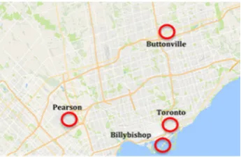
5.1 Location
321
The modeling methodology proposed in Section 4 has been applied in the case study of wind and solar
322
power systems in four sites in Central Ontario, Canada: Pearson, Toronto, BillyBishop, and Buttonville
323
(see Figure 1). These sites are important and unique due to their proximity to a densely-populated city (City
324
of Toronto) and a large water body (Lake Ontario), and their association with the main power grid in the
325
Greater Toronto Region. The power demand in this region is very high (27,000 MW /day on peak demand),
326
therefore it is critically important to achieve a stable power supply in the region. Increasing the penetration
327
of renewable energy-based systems, specifically wind power, may lead to instability in the available power
328
in the grid.
329
330
Figure 1: Central Ontario with all four locations under consideration
331
5.2 Fitting Probability Distribution Models to Wind and Solar Power Data
332
For the case study, we used data on solar power using the hourly solar insolation data for 3 years,
333
available through RETScreen [38]) and similarly data on wind power was generated using a wind turbine
334
[39] model for hourly wind speeds for 3 years for Toronto. Weibull is used as a standard for modeling wind
335
speed, log normal has been used at times as well and Gamma distribution has been sparingly used for
336
modelling solar insolation but there has been no standard distribution for fitting wind or solar power
337
generated. It is important as both wind speed and solar insolation undergo a non-linear transformation and
338
hence cannot be fit using either Weibull distribution for wind power or Gamma distribution for solar power.
339
Therefore, there is a need for a generalized distribution such as the Beta distribution that be used for fitting
340
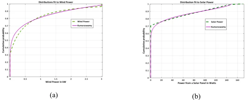
both solar and wind power. We tested the Kumaraswamy distribution for fittingboth solar power and wind
341
power data sets given its ability as a general distribution. It gives the flexibility and avoids the numerical
intractability that inhibit the use of the Beta distribution. The Kumaraswamy model best describes the
343
probability distribution of the data (see Figure 2) and hence will be used for the further study with copulas.
344
(a) (b)
Figure 2: Probability distribution models fitted to data from Toronto, Ontario for Season 3 for the three year period
345
(a) Wind Power generated from Whisper 500 3kW wind turbine (b) to solar power from a 0.18kWp solar panel
346
5.3 Analysis of Wind Power for Dependence Modeling
347
We also performed a pair-wise comparison of wind power data (by transforming the wind speed
348
information obtained from RETScreen to power using the Whisper 500 wind turbine model at each of the
349
four sites. It is a Type 1 wind turbine.) for the four sites to determine the correlation between power data at
350
the sites (see Figure 3). Since the correlations appeared non-linear and data distribution was non-Gaussian,
351
we chose Kendall rank correlation as our correlation parameter. To ensure that the wind power data were
352
non-linearly correlated, we further grouped the data set for each paired site into 3 equal subsets. For each
353
site pairing, data were randomly assigned to a sub-group. An analysis of the data correlations in the subsets
354
independently revealed that the correlations varied markedly and were not constant for the sub-groups of
355
each paired site (see Figure 3). With the exception of one sub-group for the Toronto-Pearson paired location,
356
the Kendall rank values for all other sub-groups indicate non-linear behavior. For example, the sub-plot
357
between Buttonville and BillyBishop has an overall correlation of 0.26 whereas the corresponding three
358
subsets (low, medium, and high values) have varying correlation values of 0.06, 0.23 and 0.11.
359
5.4 C-Vine Copula Generation
360
Based on the observations of wind power behavior in Section 5.3, the wind power output at each
361
site are modeled using the Kumaraswamy distribution for each of the four sites in the case study to
362
generate pair-copula construction. We employed vine copulas to model the spatial dependence of wind
363
power production sites; this choice of copula was influenced by the following factors, as seen in Figure
364
3:
365
• the wind power in each location was non-normally distributed;
366
• the Kendall rank correlations of wind power between sites varied (the correlation coefficients
367
of the subplots of Figure 3 differ); and
368
• the wind power outputs at the sites were non-linearly dependent
370
The Kumaraswamy distribution was fitted to historical wind power data from each site. Maximum
371
likelihood estimates were used to obtain the distribution parameters. To model the dependence of
372
wind power generated from the four sites with C-vine copula, we first converted the wind power data
373
from the real domain to copula data, which lie inside the [0,1] hypercube. This was accomplished by
374
taking the Kumaraswamy CDF of the individual data series.
375 376
As described earlier in Section 4.1 (Step 3), we need to identify the root node of the C-Vine tree.
377
To do this, we generated the Kendall correlation matrix for the sites and added together the correlation
378
coefficients of each site (rightmost column of Table 3). This sum is an indicator of the strength of the
379
correlation of a site’s wind power output to other locations’ wind power outputs. Consequently, the
380
site with the highest the sum is selected as the root node of the C-vine tree. In our case study, the root
381
node of the C-vine tree is the Pearsonsite.
382 383
Table 2: Kendall Correlation Matrix for the Four Sites
384 385 386 387 388 389
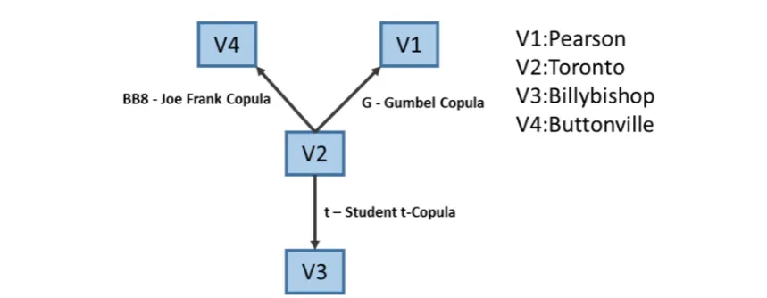
The C-vine tree representation of our power generation sites is shown in Figure 5. The three other sites
390
(Toronto, BillyBishop and Buttonville) are connected to the root node (Pearson) by a link representing the
391
pair-copula construction between the root node and the site connected to it.
392 393
We used bivariate copulas to formulate the PCC for the three links. Each link represents a copula
394
describing the dependence in the marginal distributions of wind power at each site. We used the marginal
395
distribution (Kumaraswamy distribution) for each of the three site pairs and generated scenarios of power
396
production for each site. These generated data were then used to estimate the copula parameters. The choice
397
of the copula function was based on analytical tractability and simplicity and best fit to data. Copula fitting
398
was performed in R statistical software package (R version 3.2.4) using the CDVine package. We fitted the
399
data generated from the scenarios to a set of 24 copulas using maximum likelihood estimates and ranked
400
them based on the Akaike Information Criteria (AIC) and Bayesian Information Criteria (BIC).
401 402
For each link, the copulas with the largest AIC and BIC values were chosen for that particular link.
403
Figure 6 shows the results of the copula fitting. The Gumbel copula describes the dependence of the
404
marginal distributions of wind power between Pearson and Toronto, the Student-t copula describes the
405
Pearson-BillyBishop pair, and the Joe-Frank copula describes the Pearson-Buttonville pair.
406 407
Index Toronto Pearson BillyBishop ButtonVille Sum
1 Toronto 1.000 0.811 0.561 0.213 2.585
2 Pearson 0.811 1.000 0.566 0.233 2.610
3 BillyBishop 0.561 0.566 1.000 0.255 2.382
408
Figure 3: Tree Estimated using Maximum Likelihood Estimates
409
Node labels represent the four sites in this case study: V1 (Pearson), V2 (Toronto), V3(Billybishop)
410
and V4 (Buttonville) represent the four locations in our study. Link labels represent the copula chosen for
411
modeling the spatial dependence of wind power generation between the sites based on the maximum
412
likelihood estimates: BB8 (Joe-Frank), G (Gumbel) and t (Student-t).
413 414
5.5 Optimization of Power Allocation
415
Once the model of the probability distributions of renewable power is determined (wind, using
416
Kumaraswamy distribution and copulas; and solar, using Kumaraswamy distribution) the next step is to
417
find an optimal allocation (distribution of the total capacity of solar panels and wind turbines among sites)
418
of renewable energy technologies among the four sites (see Section 4.3). Table 4 shows the results of this
419
optimization. For solar power, the distribution of weights across the four sites tends to remain constant even
420
in cases where high reliability is desired ( values range from 0.05 to 0.10). This implies low variations in
421
solar power generation across sites (i.e., stable power source). In contrast, for high reliability cases ( values
422
range from 0.05 to 0.10), wind power distributions across the four sites exhibit more pronounced variations.
423
This implies that different power allocation strategies must be implemented to achieve higher and stable
424
power output from the 4 sites.
425 426 427 428 429 430 431
Table 3: Wind and Solar Allocation Weightages
0.05 0.2556 0.2541 0.2619 0.2284 0.2498 0.2498 0.2505 0.2498
0.10 0.2670 0.2537 0.2381 0.2412 0.2500 0.2500 0.2500 0.2500
0.11 0.2486 0.2507 0.2492 0.2515 0.2500 0.2500 0.2500 0.2500
0.12 0.2499 0.2457 0.2587 0.2458 0.2500 0.2500 0.2500 0.2500
0.13 0.2529 0.2498 0.2538 0.2435 0.2485 0.2546 0.2485 0.2485
0.14 0.2609 0.2402 0.2588 0.2402 0.2486 0.2519 0.2508 0.2486
0.15 0.2551 0.2498 0.2484 0.2467 0.2496 0.2511 0.2496 0.2496
433
:Reliability factor, , , , : Weightage of allocation for wind power technology at a site and
434
, , , : Weightage of allocation for solar power technology at a site, where 1: Toronto, 2: Pearson, 435
3:Billybishop and 4: Buttonville
436
To illustrate the advantage of using this technique for allocating renewable energy technologies, we
437
compared the overall power generation (from wind and solar) when equal weightage across the four sites
438
is used, and when optimal allocation is used for = 0.05. A snapshot of power production for a 24-hour
439
period for the Season 3 months is shown in Figure 7. The optimized allocation technique results in
440
significantly higher and accurate overall power output during periods of peak power production.
441
442
Figure 7: Power production for various allocation schemes during the Season 3
444
Figure 4: Pair-wise comparison of correlations in wind power data from 4 locations in Central Ontario. In the plots above the figures in black in each sub-plot represents the correlation coefficient for the entire data. Besides Pearson vs Toronto all other datasets are highly non-linear. Pink lines are least-square regression line whose slope is the correlation coefficient for the entire dataset. The panels in the main diagonal represent the histograms of the variables.
6. Conclusions
446
Copulas are one of the most sophisticated tools for modeling the dependence structure of
447
between variables when their correlation is non-linear. In this paper, we present a methodology for
448
modeling the non-linear spatial dependence in wind power generation using copulas. We modeled
449
the temporal distributions of both wind and solar power for each individual location using the
450
Kumaraswamy distribution. The data for solar and wind power generated from these probabilistic
451
models is used in an optimization model for obtaining an appropriate allocation of solar and wind
452
power technologies in a spatially dispersed landscape to maximize the overall power output and
453
minimize the effect of random nature of the renewable sources of energy. We find that this approach
454
is useful in increasing the overall reliability of energy production as well as accurate modeling of
455
renewable resources.
456
Acknowledgement
457
This work was supported by the Natural Sciences and Engineering Research Council of Canada
458
(NSERC). NSERC had no inputs in the study design, model development and implementation, and
459
in the preparation of this manuscript.
460
References
461
1. D.E. Newton, World Energy Crisis: A Reference Handbook, ABC-CLIO, 2013 .
462
2. K. GILLINGHAM and J. SWEENEY, "BARRIERS TO IMPLEMENTING LOW-CARBON
463
TECHNOLOGIES," Climate Change Economics, vol. 03, pp. 1250019, 2012.
464
3. F. Ribeiro, P. Salgado and J. Barreira, "Engineering Applications of Neural Networks: 13th International
465
Conference, EANN 2012, London, UK, September 20-23, 2012. Proceedings," pp. 254-263, 2012.
466
4. D.L. King, W.E. Boyson and J.A. Kratochvil, "Analysis of factors influencing the annual energy production
467
of photovoltaic systems," in Photovoltaic Specialists Conference, 2002. Conference Record of the
Twenty-468
Ninth IEEE, pp. 1356-1361, 2002.
469
5. T. Hammons, "Integrating renewable energy sources into European grids," International Journal of
470
Electrical Power & Energy Systems, vol. 30, pp. 462-475, 2008.
471
6. O. Grothe and J. Schnieders, "Spatial dependence in wind and optimal wind power allocation: A
copula-472
based analysis," Energy Policy, vol. 39, pp. 4742-4754, sep. 2011.
473
7. B. Hasche, "General statistics of geographically dispersed wind power," Wind Energy, vol. 13, pp. 773-784,
474
2010.
475
8. A. Gerber, M. Qadrdan, M. Chaudry, J. Ekanayake and N. Jenkins, "A 2020Â GB transmission network
476
study using dispersed wind farm power output," Renewable Energy, vol. 37, pp. 124, 2012.
477
9. E. Kahn, "The reliability of distributed wind generators," Electr.Power Syst.Res., vol. 2, pp. 1, 1979.
478
10. A. Abdollahi and M.P. Moghaddam, "Investigation of Economic and Environmental-Driven Demand
479
Response Measures Incorporating UC," IEEE Transactions on Smart Grids, vol. 3, pp. 12-25, 2012.
480
11. D. D. Le, G. Gross and A. Berizzi, "Probabilistic Modeling of Multisite Wind Farm Production for
Scenario-481
Based Applications," IEEE Transactions on Sustainable Energy, vol. 6, pp. 748-758, July. 2015.
482
12. K. Veeramachaneni, X. Ye and U. O’Reilly, "Statistical Approaches for Wind Resource Assessment,"
483
Computational Intelligent Data Analysis for Sustainable Development, pp. 303, 2013.
484
13. D. P. Kroese, T. Taimre and Z.I. Botev, Handbook of Monte Carlo Methods, Wiley, 2013, .
485
14. J. S. Benth and F.E. Benth, "Analysis and modelling of wind speed in New York," Journal of Applied
486
Statistics, vol. 37, pp. 893-909, 2010.
487
15. R. T. Clemen and T. Reilly, "Correlations and Copulas for Decision and Risk Analysis," Management
488
Science, vol. 45, pp. 208-224, 1999.
Renewable Energy, vol. 35, pp. 1991-2000, 9. 2010.
492
17. S. Hagspiel, A. Papaemannouil, M. Schmid and G. Andersson, "Copula-based modeling of stochastic wind
493
power in Europe and implications for the Swiss power grid," Appl.Energy, vol. 96, pp. 33, 2012.
494
18. G. Papaefthymiou and D. Kurowicka, "Using Copulas for Modeling Stochastic Dependence in Power
495
System Uncertainty Analysis," Power Systems, IEEE Transactions On, vol. 24, pp. 40-49, Feb. 2009.
496
19. R.B. Nelsen, An introduction to copulas, New York : Springer, c2006, 2006, .
497
20. P. Joubert, "Modelling Copulas : An Overview," pp. 1-27, .
498
21. Yih-Huei Wan, "Wind power plant behaviors: Analyses of long-term wind power data," NREL., Tech. Rep.
499
NREL/TP-500-36551, 2004.
500
22. Bernhard Ernst, Yih-Huei Wan, Brendan Kirby, "Short-term power fluctuation of wind turbines: Analyzing
501
data from the German 250-MW measurement program from the ancillary services viewpoint," NREL.,
502
Tech. Rep. NREL/CP-500-26722, 1999.
503
23. H. Louie, "Evaluating Archimedean Copula models of wind speed for wind power modeling," in Power
504
Engineering Society Conference and Exposition in Africa (PowerAfrica), 2012 IEEE, pp. 1-5, 2012.
505
24. P. Pinson and R. Girard, "Evaluating the quality of scenarios of short-term wind power generation,"
506
Appl.Energy, vol. 96, pp. 12, 2012.
507
25. S. Gill, B. Stephen and S. Galloway, "Wind Turbine Condition Assessment Through Power Curve Copula
508
Modeling," Sustainable Energy, IEEE Transactions On, vol. 3, pp. 94-101, Jan. 2012.
509
26. R. J. Bessa, J. Mendes, V. Miranda, A. Botterud, J. Wang and Z. Zhou, "Quantile-copula density forecast for
510
wind power uncertainty modeling," in PowerTech, 2011 IEEE Trondheim, pp. 1-8, 2011.
511
27. D. Heinemann, E. Lorenz and M. Girodo, "Forecasting of solar radiation," Solar Energy Resource
512
Management for Electricity Generation from Local Level to Global Scale.Nova Science Publishers, New
513
York, 2006.
514
28. G. Tina, S. Gagliano and V.A. Doria, "Probability Analysis of Weather Data for Energy Assessment of
515
Hybrid Solar / Wind Power System University of Catania," in 4th IASME/WSEAS Interantional Conference
516
on ENERGY, ECOSYSTEMS and SUSTAINABLE DEVELOPEMNT, pp. 217-223, 2008.
517
29. A. Sfetsos, "A comparison of various forecasting techniques applied to mean hourly wind speed time
518
series," Renewable Energy, vol. 21, pp. 23-35, 2000.
519
30. B. Tarroja, F. Mueller and S. Samuelsen, "Solar power variability and spatial diversification: implications
520
from an electric grid load balancing perspective," Int.J.Energy Res., vol. 37, pp. 1002-1016, 2013.
521
31. A. Seifi, K. Ponnambalam and J. Vlach, "A unified approach to statistical design centering of integrated
522
circuits with correlated parameters," Circuits and Systems I: Fundamental Theory and Applications, IEEE
523
Transactions On, vol. 46, pp. 190-196, Jan. 1999.
524
32. A. Seifi, K. Ponnambalam and J. Vlach, "Optimization of filter designs with dependent and asymmetrically
525
distributed parameters," Journal of the Franklin Institute, vol. 350, pp. 378, 2013.
526
33. A. Sklar, "Distribution functions of n dimensions and margins," Publications of the Institute of Statistics of
527
the University of Paris, vol. 8, pp. 229-231, 1959.
528
34. W. Hurlimann, "Fitting bivariate cumulative returns with copulas," Computational Statistics \& Data
529
Analysis, vol. 45, pp. 355-372, 2004.
530
35. H. Joe, Multivariate Models and Multivariate Dependence Concepts, Taylor \& Francis, 1997, .
531
36. T. Bedford and R. Cooke, Probabilistic Risk Analysis: Foundations and Methods, Cambridge University
532
Press, 2001, .
533
37. K. Aas, C. Czado, A. Frigessi and H. Bakken, "Pair-copula constructions of multiple dependence,"
534
Insurance: Mathematics and Economics, vol. 44, pp. 182-198, 2009.
535
38. G. J. Leng, A. Monarque, R. Alward, N. Meloche and A. Richard, "Canada's Renewable Energy Capacity
536
Building Program & Retscreen International," in Proceedings of the World Renewable Energy Congress
537
VII, Cologne, Germany, 2002.
538
39. Southwest Energy, "Specification Sheet Whisper 500,"