A study of photon structure with special attention to the low-x region

A S tu d y o f P h o to n

S tru ctu re w ith Special

A tten tio n to th e Low-j; R egion

J. Jason W ard

D ep artm en t of Physics and A stronom y U niversity College London

Subm itted for th e degree of D o cto r o f P h ilo so p h y

ProQuest Number: 10018676

All rights reserved

INFORMATION TO ALL USERS

The quality of this reproduction is dependent upon the quality of the copy submitted.

In the unlikely event that the author did not send a complete manuscript and there are missing pages, these will be noted. Also, if material had to be removed,

a note will indicate the deletion.

uest.

ProQuest 10018676

Published by ProQuest LLC(2016). Copyright of the Dissertation is held by the Author.

All rights reserved.

This work is protected against unauthorized copying under Title 17, United States Code. Microform Edition © ProQuest LLC.

ProQuest LLC

789 East Eisenhower Parkway P.O. Box 1346

A b stra ct

A cknow ledgem ents

First and forem ost I would like to thank David Miller for his supervision and support throughout this work. I am indebted to Bruce Kennedy and M ark Lehto who both helped to get me going w ith the analysis.

The OPAL C ollaboration are gratefully acknowledged for their hard work in building and run­ ning the detector which provides the d a ta for this thesis. Special thanks to Jim Conboy, Allan Skillman, Ed McKigney, Tony Rooke, Joerg Bechtluft, Bernd W ilkens, Steve Hillier, R ichard Nisius, Volker Blobel and Peter Hobson who have all been fine collaborators. My understanding of the theory of tw o-photon physics is much b etter after discussions with Jeff Forshaw, and Mike Seymour has been excellent with answering my HERW IG questions.

Thanks to David Munday, T ara Shears, Bill Allison and G uy Pooley, who all helped me when I was applying to various places to do a Ph.D . - all of the support and encouragement th a t I got m ade a big difference.

For financial support I would like to thank the Particle Physics and Astronom y Research Council and University College London. Also the University of London’s award of the 1994 Valerie Myerscough Prize m ade a trip to a NATO Advanced Study In stitu te possible.

During the P h.D ., and because of it, I was fortunate enough to become involved in two new activities th a t have shown ways towards having a quiet m ind. A bow to Dennis Ngo for being an excellent teacher of T a i’ Chi (Suan Yang of the T iger-C rane com bination) and an enormous thankyou to Paul Phillips and C hristine Beeston for getting me into m ountain walking.

Special thanks to Ja n Lauber, W arren M atthews, M ark Lehto (again!), M ark Pearce, Kwasi Ametewee, Nick Feast, Harvey May cock, K atrijn R aaij m akers and Philippe Persiaux, who have all provided alot of support on various occasions.

Finally, thanks to m y parents, M argaret and John W ard, and my sisters, Hayley and Michelle W ard, for their continuing Love and support.

This thesis is dedicated to all of the people nam ed above. It could not have been produced w ithout them .

C on ten ts

L ist o f Figures 8

List o f Tables 15

1 Introd u ction 17

1.1 Tw o-Photon I n te r a c tio n s ... 18

1.2 T he Photon P i c t u r e ... 18

1.3 The e7 V e r te x ... 19

1.4 7 7 Collisions at an e+e" C o l l i d e r ... 19

1.5 Deep Inelastic e7 S c a t t e r i n g ... 21

1.6 Interest in ... 23

1.7 FJ M easurem ents a t L E P ... 28

2 T h eory o f th e P h o to n S tru ctu re Function 31 2.1 P arto n D istributions of th e P h o t o n ... 31

2.2 T he Com ponents of ... 32

2.3 Vector Meson D om inance ... 33

2.4 T he Q uark P a rto n M odel ... 34

C O N T EN T S 5

2.5.1 T he D G LA P Evolution E q u a tio n s ... 37

2.5.2 P arto n D istributions at L o w - z ... 38

2.6 C h arm -Q u ark C o n trib u tio n s ... 39

2.7 F2 P aram eterisatio n s and M o d e l s ... 42

2.7.1 Glück, R eya and Vogt ( G R V ) ... 42

2.7.2 H agiw ara et al. ( W H I T ) ... 43

2.7.3 G ordon and Storrow ( G S ) ... 43

2.7.4 Drees and Grassie ( D G ) ... 44

2.7.5 Levy, Abram owicz and C harcula (LAC) ... 45

2.7.6 A urenche et al. ( A C F G P ) ... 45

2.7.7 Field, K ap u sta and Poggioli ( F K P ) ... 47

2.7.8 Schuler and Sjôstrand ( S a S ) ... 48

3 LE P and th e O PAL D e te c to r 50 3.1 L E P ... 50

3.2 T he OPAL D e t e c t o r ... 51

3.2.1 C entral Tracking D e te c to rs ... 54

3.2.2 Tim e-of-Flight ... 56

3.2.3 E lectrom agnetic C a lo rim e try ... 56

3.2.4 H adron C a lo rim e te r... 59

3.2.5 M uon D e t e c t o r ... 59

3.3 OPAL Forward D e t e c t o r s ... 60

3.3.1 Silicon T ungsten C alorim eter ( S W ) ... 60

3.3.2 Forward D etector ( F D ) ... 60

6 C O N T E N T S

4 E ven t S electio n 68

4.1 Event S e l e c t i o n ... 68

4.1.1 P r e s e le c tio n ... 69

4.1.2 F u rth er S e l e c t i o n ... 70

4.1.3 Final S e l e c t i o n ... 72

4.2 E stim atio n of B ac k g ro u n d s... 75

4.2.1 e‘^e“ —>• hadrons ... 75

4.2.2 e + e " ^ r + r “ 75 4.2.3 N o n -m ultiperipheral e+e“ ->-e‘*'e” + hadrons ... 75

4.2.4 B eam -gas e v e n t s ... 78

4.3 Trigger E ffic ie n c y ... 78

4.3.1 C alculation of E f fic ie n c y ... 78

4.3.2 E stim atio n of Efficiency from th e D a t a ... 79

4.4 D a ta Self Consistency ... 80

5 M on te C arlo S im u lation 91 5.1 7*7 F r a g m e n ta t io n ... 92

5.2 V e r m a s e r e n ... 92

5.3 F2G EN ... 92

5.4 H E R W I G ... 94

5.5 C om parison of G e n e r a t o r s ... 97

5.6 M onte Carlo Samples G e n e ra te d ... 99

6 C om parison o f D a ta w ith M o n te Carlo 102 6.1 M onte Carlo Models in th e C o m p a ris o n ... 103

C O N T E N T S 7

6.3 S u m m a r y ... 126

7 U n fold in g 127 7.1 T he Problem of M easuring 77^(2: ) ... 127

7.2 T he Forward M e t h o d ... 128

7.3 T he Inverse M ethod ... 130

7.4 D is c r e tiz a tio n ... 131

7.5 U n f o l d i n g ... 131

7.6 Unfolding Exam ples ... 134

7.6.1 Unfolding in a B i n ... 135

7.6.2 T he Unfolding T e s t s ... 136

7.7 D ata U n fo ld in g s... 143

8 S u m m ary and C onclusions 157

List o f Figures

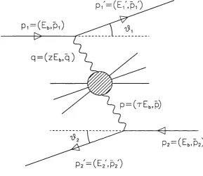
1.1 T he m ulti-peripheral tw o-photon process labelled w ith four-vectors, z and T are th e energies of th e probing and probed photon respec­ tively, expressed as a fraction of th e beam energy... 20

1.2 C om parison of evolution of th e second m om ent of in QCD (solid line) w ith a theory in which th e coupling constant is frozen a t an initial value of Qg = 5 GeV^ (dot-dashed line)... 25

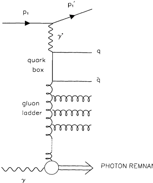
1.3 Feynm an diagram used in some QCD models of th e low-a; p a rt of th e photon stru ctu re fu n ctio n... 26

1.4 Rise in th e proton stru c tu re function m easured by th e ZEUS Col­ laboration (circles) and th e H I C ollaboration (triangles)... 27

1.5 S catter plot of M onte Carlo tagged tw o-photon events from the F2GEN generator (see Section 5.3) at Ebeam = 45.6 GeV. T he m in­ im um 7 7 m ass is 2 GeV, th e m inim um tag angle is 30 m rad and th e m inim um tag energy is 20 GeV. T he photonic parto n distrib u tio n functions from GRV (see Section 2.7.1) have been used in th e event generation... 30

2.1 Q PM and VMD predictions for • T he simple VMD and T P G/2 7

VMD predictions are from E quations 2.8 and 2.10 respectively. The Q PM prediction (E quation 2.13) are for 3 flavours, w ith = rrid = ms = 300 M eV ... 35 2.2 T he T P C/2 7 VMD prediction is shown by th e do tted line. The

L I S T OF FIGURES 9

2.3 The GRV Leading O rder param eterisatio n for four flavours (solid lines) and three flavours (dashed lines). T he lower curve of each pair is calculated a t Q ^=5.9 GeV^ and th e upper curve of each pair is calculated a t (5^=14.7 GeV^... 41

2.4 The LA C l param eterisatio n for four flavours (solid lines) and th ree flavours (dashed lines). T h e lower curve of each pair is calculated at Q^=5.9 GeV^ and th e u p p er curve of each pair is calculated at Q "=14.7 GeV"... 46

2.5 A selection of three-flavour F^i^x) param eterisations from Section 2.7. All of these curves are calculated a t Q^=14.7 G eV"... 49

3.1 A cut-away view of th e OPAL d e tec to r... 52

3.2 Side and end views of th e OPAL detector, sectioned to show th e m ain subdetector system s: central vertex cham ber, je t cham ber and z-cham bers (CV, CJ and CZ), electrom agnetic calorim eters (EB and EE), hadron calorim eters (HB and HE) and m uon cham bers (MB and M E). T he forw ard detector m odules (FD ) can also be seen. 53

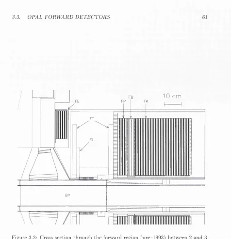
3.3 Cross section through th e forward region (pre-1993) betw een 2 and 3 m etres from th e intersection region (which is to th e left of this diagram ). BP = B eam P ip e, ET = D rift C ham bers, EL = Fine Lum inosity M onitor, EE = G am m a C atcher, F P = P resam pler C alorim eter, FB = Tube C ham bers and FK = M ain C alorim eter. 61

?eam •

4.1 E stim ate of background events, (a) D istribution in Etag/Eb^ The vertical d o t-d ash ed line shows where th e m inim um tag energy cut is. (b) The d istrib u tio n in Xyis after all of th e selection cuts have been applied. T he background estim ate in th is histogram is enhanced by a factor of 10... 76

4.2 T he four m ain diagram s contributing in th e lowest order to th e process 7 7 . These processes are included in PE R M ISV. U nlabelled boson lines represent photons only... 77

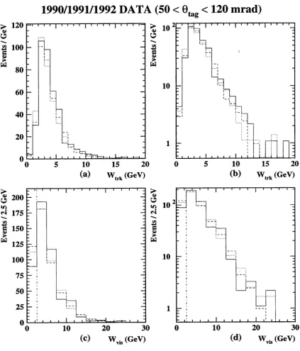
4.3 Comparison of 1990 (solid), 1991 (dashed) and 1992 (d o tted ) tag distributions. Final selection cuts are represented by vertical d o t- dashed lines... 83

10 L IS T OF FIGURES

4.5 C om parison of 1990 (solid), 1991 (dashed) and 1992 (dotted) in­ variant m ass distributions. Final selection cuts are represented by vertical d o t-d ash ed lines... 85

4.6 C om parison of 1990 (solid), 1991 (dashed) and 1992 (dotted) an ti­ tag and n eu tral energy distributions. Final selection cuts are rep­ resented by vertical d o t-d ash ed lines... 86

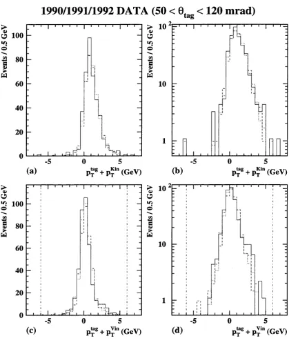
4.7 Com parison of 1990 (solid), 1991 (dashed) and 1992 (dotted) tra n s­ verse m om entum distributions (defined in Section 4.1.3) in th e plane of th e beam and th e tag. Final selection cuts are represented by vertical d o t-d ash ed lines... 87

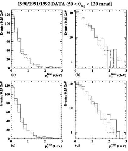
4.8 C om parison of 1990 (solid), 1991 (dashed) and 1992 (dotted) tra n s­ verse m om entum distributions (defined in Section 4.1.3) out of th e plane of th e beam and th e ta g ... 88

4.9 Com parison of 1990 (solid), 1991 (dashed) and 1992 (dotted) tra n s­ verse m om entum distributions (defined in Section 4.1.3) out of the plane of th e beam and th e tag. ... 89

4.10 C om parison of 1990 (solid), 1991 (dashed) and 1992 (dotted) track m ultiplicity distributions. Final selection cuts are represented by vertical d o t-d ash ed lines... 90

5.1 A representation of th e deep inelastic 67 scattering process in th e H ERW IG M onte Carlo. ISPS and FSPS are th e initial and final sta te p arto n showers respectively... 96

6.1 Tag d istributions for th e d a ta (dots) and th e M onte Carlo models in th e whole 9tag range. T he different samples are from F2GEN GRV 100% p o in t-lik e (solid), F2G EN GRV ‘perim iss(O .l)’ (dashed), H ER ­ W IG GRV w ithout th e SUE (d o tted) and HERW IG LA C l w ithout th e SUE (d o t-d ash e d )... 105

6.2 Xtrk-, ^vis and XyisFD distributions (each defined in Section 4.1.2) for th e d a ta (dots) and th e M onte Carlo models in th e low Otag range. T he different samples are from F2G EN GRV 100% po in t­ like (solid), F2GEN GRV ‘perim iss(O .l)’ (dashed), HERW IG GRV w ithout th e SUE (dotted) and HERW IG LA C l w ithout th e SUE

L IS T OF FIGURES 11

6.3 Xtrk, ^vis and XyisFD distributions (each defined in Section 4.1.2) for th e d a ta (dots) and the M onte Carlo models in th e high Otag range. T he different samples are from F2G EN GRV 100% point­ like (solid), F2G EN GRV ‘perim iss(O .l)’ (dashed), HERW IG GRV w ithout th e SUE (dotted) and HERW IG LA C l w ithout th e SUE (d o t-d a sh e d )... 107

6.4 Invariant m ass distributions for th e d a ta (dots) and th e M onte Carlo m odels in th e low Otag range. T he different samples are fro m , F2G EN GRV 100% p o int-lik e (solid), F2G EN GRV ‘perim iss(O .l)’ (dashed), HERW IG GRV w ithout th e SUE (do tted ) and HERW IG LA Cl w ithout th e SUE (d o t-d ash e d )... 108

6.5 Invariant mass distributions for th e d a ta (dots) and th e M onte Carlo m odels in th e high Otag range. T he different samples are from F2G EN GRV 100% point-like (solid), F2G EN GRV ‘perim - iss(O .l)’ (dashed), HERW IG GRV w ithout th e SUE (dotted) and HERW IG LA C l w ithout the SUE (d o t-d a sh e d )... 109

6.6 Xyisjxtrue Correlation plots from th e F2G EN and HERW IG M onte Carlo m odels in th e low Otag range. T he different samples are from F2G EN GRV 100% point-like (solid lines, closed circles), F2GEN GRV ‘perim iss(O .l)’ (dashed lines, open circles), HERW IG GRV w ithout th e SUE (dotted lines, closed squares) and HERW IG GRV w ith th e SUE (d o t-dash ed lines, open squares)... 112

6.7 Xyis/xtrue Correlation plots from th e F2G EN and H ERW IG M onte Carlo m odels in th e high Otag range. T h e different samples are from F2G EN GRV 100% point-like (solid lines, closed circles), F2GEN GRV ‘perim iss(O .l)’ (dashed lines, open circles), HERW IG GRV w ithout th e SUE (d o tted lines, closed squares) and HERW IG GRV w ith th e SUE (d o t-d ash ed lines, open squares)... 113

6.8 A n ti-ta g and n eu tral energy distributions for th e d a ta (dots) and th e M onte Carlo models in th e low Otag range. T he different sam­ ples are from F2G EN GRV 100% p o in t-lik e (solid), F2G EN GRV ‘perim iss(O .l)’ (dashed), HERW IG GRV w ithout th e SUE (dotted) and H ERW IG LA C l w ithout th e SUE (d o t-d a sh e d )... 115

12 L IS T OF FIGURES

6.10 Transverse m om entum distributions (defined in Section 4.1.3) in th e plane of th e beam and th e tag for th e d a ta (dots) and th e M onte Carlo models in th e low Ofag range. The different sam ples are from F2GEN GRV 100% p oin t-lik e (solid), F2GEN GRV ‘perim iss(O .l)’ (dashed), H ERW IG GRV w ithout th e SUE (dotted) and HERW IG LA C l w ithout th e SUE (d o t-d ash e d )... 117

6.11 Transverse m om en tu m distributions (defined in Section 4.1.3) in th e plane of th e beam and th e tag for th e d a ta (dots) and th e M onte Carlo models in th e high $tag range. The different samples are from F2G EN GRV 100% p o in t-like (solid), E2GEN GRV ‘perim iss(O .l)’ (dashed), HERW IG GRV w ithout th e SUE (dotted) and HERW IG LA C l w ithout th e SUE (d o t-d ash e d )... 118

6.12 Transverse m om entum distributions (defined in Section 4.1.3) out

of th e plane of th e beam and th e tag for th e d a ta (dots) and th e M onte Carlo m odels in th e low $iag range. The different samples are from E2GEN GRV 100% point-like (solid), F2G EN GRV ‘per- im iss(O .l)’ (dashed), HERW IG GRV w ithout th e SUE (dotted) and HERW IG LA C l w ithout th e SUE (d o t-d ash ed )... 119

6.13 Transverse m om entu m distributions (defined in Section 4.1.3) out of the plane of th e beam and th e tag for th e d a ta (dots) and the M onte Carlo m odels in th e high Otag range. The different samples are from F2GEN GRV 100% point-like (solid), F2G EN GRV ‘per- im iss(O .l)’ (dashed), HERW IG GRV w ithout the SUE (dotted) and HERW IG LA C l w ithout th e SUE (d o t-d ash ed )... 120

6.14 Transverse m om entum distributions (defined in Section 4.1.3) out of th e plane of th e beam and th e tag for th e d a ta (dots) and the M onte Carlo m odels in th e low Otag range. The different samples are from F2G EN GRV 100% point-like (solid), E2GEN GRV ‘per- im iss(O .l)’ (dashed), H ERW IG GRV w ithout the SUE (dotted) and HERW IG L A C l w itho u t th e SUE (d o t-d ash ed )... 121

LIST OF FIGURES 13

6.16 Track m ultiplicity, energy and energy flow d istributions for th e d a ta (dots) and th e M onte Carlo m odels in th e low Otag range. T he different sam ples are from F2G EN GRV 100% poin t-lik e (solid), F2G E N GRV ‘perim iss(O .l)’ (dashed), HERW IG GRV w ithout th e SUE (d o tted ) and HERW IG LA C l w ithout th e SUE (d o t-d ash ed ). 124

6.17 Track m ultiplicity, energy and energy flow distributions for th e d a ta (dots) and th e M onte Carlo m odels in th e high Otag range. T he different sam ples are from F2G EN GRV 100% poin t-lik e (solid), F2G EN GRV ‘perim iss(O .l)’ (dashed), HERW IG GRV w ithout th e SUE (d o tted ) and HERW IG LA C l w ithout th e SUE (d ot-d ash ed ). 125

7.1 H istogram and profile plot of Xyig and Xtme- T he HERW IG M onte Carlo has been used w ith th e GRV and w ithout th e soft under­ lying event. T he events have passed th e analysis cuts w ith tags for all of th e Otag region (50-120 m rad). T he vertical error bars on th e profile plot represent the error on th e m e an ... 129

7.2 Test unfoldings each using th e H ERW IG generator w ith th e GRV F 7 (^ ) {without th e soft underlying event) as th e unfolding M onte Carlo, (a) and (b) use th e HERW IG GRV F^(a;) without th e soft underlying event as th e “d a ta ” , (c) and (d) use th e HERW IG GRV F2 {x) with th e soft underlying event as th e “d a ta ” . Solid

lines represent th e unfolded results and th e horizontal d o tted lines represent th e GRV expectation values for each unfolded bin. . . . 139

7.3 Test unfoldings each using th e H ERW IG generator w ith th e GRV F y (^ ) th e unfolding M onte Carlo. T he “d a ta ” in each case come from HERW IG w ith the LA C l F ^ ix ). B oth th e unfolding M onte C arlo and th e “d a ta ” are w ithout th e soft underlying event. Xyis for b o th “d a ta ” and M onte Carlo is calculated without FD clusters in (a) and (b); with FD clusters in (c) and (d). Solid lines represent th e unfolded results and th e horizontal d o tted lines represent th e LA C l expectation values for each unfolded b in ... 140

14 LIST OF FIGURES

7.5 X distributions for d a ta and M onte Carlo in th e high 9tag region. T he d a ta distributions are represented by the dots. The differ­ ent M onte C arlo sam ples are from F2GEN GRV 100% point-like (solid line), F2GEN GRV ‘perim iss(O .l)’ (dashed line), HERW IG GRV w ithout th e SUE (d otted line) and HERW IG GRV w ith the SUE (d o t-d ash ed lin e)... 145

7.6 Four-flavour unfoldings of th e d a ta w ith different M onte Carlo models in th e low Otag region. T he dashed line is th e four-flavour GRV p aram eterisatio n calculated at = 5.9 GeV^, which has been included for reference only... 147 7.7 Four-flavour unfoldings of th e d a ta w ith different M onte Carlo

models in th e high Otag region. The dashed line is the four-flavour GRV p aram eterisatio n calculated at = 14.7 GeV^, which has been included for reference only... 148 7.8 C om bined four-flavour unfoldings of th e d a ta in th e low Otag region.

T he inner error bars are statistical only. T he outer error bars are th e statistical and system atic errors combined in quadrature. The broken lines are th e four-flavour GRV (dashed) and LACl (dotted) p aram eterisatio n s calculated at = 5.9 GeV^... 150 7.9 C om bined four-flavour unfoldings of th e d a ta in th e high Otag re­

gion. T he inner error bars are statistical only. The outer error bars are th e statistic a l and system atic errors combined in quadrature. T he broken lines are th e four-flavour GRV (dashed) and LACl (d o tted ) param eterisatio n s calculated at = 14.7 GeV^... 151 7.10 Com parison in th e low region of th e combined four-flavour

result of this thesis, unfolded on a log^g a; scale, w ith the th re e - flavour OPAL [34] result (w ith an estim ate of th e charm contribu­ tion added) unfolded on a linear x scale... 153 7.11 Com parison in th e high region of th e combined four-flavour

result of this thesis, unfolded on a log^g ^ scale, w ith three-flavour OPAL [34] and D E L PH I [36] results (w ith an estim ate of th e charm contribution added) unfolded on a linear x scale... 154 7.12 Com parison in th e high region of th e combined four-flavour

15

List o f Tables

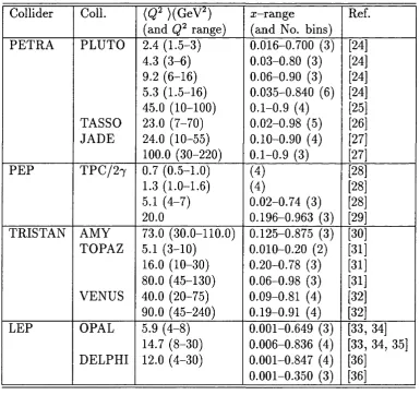
1.1 Published hadronic Fo d a ta as a function of a;... 28

3.1 Sum m ary of triggers used in triggering tagged tw o-photon events, w ith typical threshold values. T he superscript S indicates a stan ­ dalone trigger and th e superscript C indicates th a t th e trigger forms p a rt of th e C EN TR L trigger described in Section 4.3.2. T he n o ta­ tion L(R) refers to th e Left (R ight) sides of O PA L... 66

3.2 Program m ed trigger conditions combining triggers from tag and hadronic activity in tagged tw o-photon events... 67

4.1 Q uality cuts applied to th e tracks, n eu tral clusters and th e track-cluster association cone. T he quantities are described in Section 4.1.2. 69

4.2 D etector statu s num ber and in te rp re ta tio n ... 70

4.3 Final selection cuts. T he quantities are described in Section 4.1.3. 73

4.4 M easured trigger efficiencies... 79

4.5 Com parison of num b er of events, integrated lum inosities and cross-sections for th e selection cuts in 1990, 1991 and 1992. T he num bers in brackets indicate th e num bers of events for th e Otag regions of 50-70 m rad and 70-120 m rad respectively. T he trigger efficiency is accounted for in th e calculation of th e cross-section for th e cuts. . 80

16 LIST OF TAB LES

5.2 M onte Carlo generated sam ples th a t have had the full OPAL de­ te cto r sim ulation (GOPAL) applied to them . The d a ta have been included a t th e b o ttom of th e tab le for comparison w ith th e M onte Carlo. T he num bers in brackets indicate th e cross-sections for the 0tag regions of 50-70 m rad an d 70-120 m rad respectively... 101

7.1 M onte Carlo samples generated by HERW IG for unfolding tests. In each entry, th e first line is th e unfolding M onte Carlo and th e second line is th e mock d ata. F u rth er explanation of this tab le is given in Section 7.6.2... 137 7.2 Four-flavour unfoldings of th e d a ta w ith different M onte Carlo

models in th e low Otag region... 149 7.3 Four-flavour unfoldings of th e d a ta w ith different M onte Carlo

17

C hapter 1

In tro d u ctio n

This thesis is a study of singly-tagged tw o-photon collisions using d a ta from th e OPAL (O m n i-P u rp o se A p p aratu s for LEP) detecto r [1] a t th e LEP (Large E lectron-P ositron) collider [2] at CERN near Geneva. T he aim of such a study is to obtain a m easurem ent of th e hadronic photon stru c tu re function, E^(T, Q^).

T he d a ta used in this analysis were taken in th e years 1990-1992 and correspond to 45.93 p b “ ^ of e'*'e“ in teg rated luminosity.

As an introduction it is acknowledged th a t th e photon has a hadronic structure. A sim ple picture for this stru c tu re is presented, followed by th e m ethod used to stu d y this stru ctu re at an e+ e" collider. T he photon stru c tu re function is then introduced and th e m otivation for m easuring it is given.

18 CH APTER 1. I NT RO DUC TI ON

1.1

T w o-P hoton Interactions

In classical electrodynam ics th e photon is described by th e linear Maxwell equa­ tions. However, in quantum m echanics, th e photon is not a photon all of th e tim e. A photon of energy can flu ctu ate into a virtu al sta te of a charged particle pair, by th e un certain ty principle. If nipair is th e m ass of th e charged particle pair, then th e lifetim e of th e state is given by

2E

(1.1)

TOp«.V

assum ing <K E^ and h = c = 1. This tim e increases as th e photon energy increases. Therefore, an in teractio n of two photons becomes possible because one photon can in teract w ith one of th e charged particles in th e state th e oth er photon has fluctuated into.

1.2

T he P h oton P ictu re

T he virtu al sta te of th e charged p article pair can be either a charged lepton- an tilep to n pair (/"'■/“ ), a q u ark-antiquark pair {qq ) or a m assive p air (e.g. W '^ W ~ ) . A cut-off param eter po m ay be introduced to separate th e range of 7 —>• çç fluctu­ ations into low- and high-virtuality states. Such a separation is necessary because th e low -virtuality state is in th e regim e of non-perturbative QCD physics. The vector m eson dom inance (VM D) m odel approxim ates th e range of 7 —> gq fluc­ tu atio n s below Po by a sum over low -m ass vector meson states. Each meson state can be w ritten as |V). po sets th e m inim um transverse m om entum of th e qq p air in th e high-virtuality p e rtu rb a tiv e p a rt of 7 —>■ çg fluctuations (th e so-called ‘p o in t-lik e’ com ponent). This s ta te can be w ritten as \qq). T he com plete photon wave-function for low-m ass states [3] is th en

b ) = Cbarellbare) A ^ | V) -f ^ C, -f ^ Q |/+/ ). (1.2)

1.3. T H E Eq V E R T E X 19

1.3

T he 87 V ertex

By th e u n certain ty principle an electron of energy Eb can fluctuate into a v irtu al electron-photon state. This is illu strated in th e top vertex of Figure 1.1. If th e electron is scattered w ith energy E[ into a solid angle elem ent dfl, at angle 6i to th e in itial electron direction, after producing a photon of energy zEb th en th e flux for such a process is given by [4]

( U )

aem is th e electrom agnetic coupling constant and which is by deflnition th e negative of th e four-m om entum squared of th e photon, is given by

= _ g2 ^ 4EbE[ sin^ (1.4)

where th e m ass of th e electron has been neglected. It should be noted th a t th e above flux factor peaks at small values of and small photon energies.

1.4

77 C ollisions at an e^e Collider

T he only way of studying photon stru c tu re a t current e'^'e" colliders is to use an e7 vertex from one electron (positron) to produce a nearly-real photon th a t will display th e stru c tu re described in Section 1.2. A second photon of high virtu ality from th e eq vertex of th e opposing positron (electron) can be used to probe th e s tru c tu re of th e nearly-real photon. T he m ulti-peripheral tw o-photon process is illu strated in Figure 1.1. It is custom ary to label th e four-vector of th e v irtu al probe photon as q and th e four-vector of th e nearly-real photon as p. T he invariant kinem atic variables

91_____ (1 5 )

2 p - q Q^ + P^ + W ^ ^ ^

20 C H A P T E R 1. INTRODUCTION

1.5. DEEP IN EL A S T IC Ey S C A T T E R IN G 21

can be defined w ith reference to th e four-vectors in Figure 1.1. VF is th e invariant mass of th e tw o-photon system . T w o-photon collisions where one photon is v irtu al and one is real will be called ‘7*7 collisions’. T he * m arks th e highly v irtu al photon.

1.5

D eep Inelastic

e j

Scattering

W hen ^ 4 GeV^ and ~ 0 th e tw o-photon collision can be regarded as deep-inelastic electron-photon scattering, where th e bare probe photon couples to a quark inside th e nearly-real photon resulting in an hadronic final state. E xperi­ m entally, deep inelastic e j scattering is observed w ith singly-tagged events, where th e probe photon has its determ ined from th e energy (E[) and angle (^1) of th e scattered electron (called th e ‘ta g ’) and ~ 0 is ensured by requiring th a t th e positron is not seen in th e detector (called th e ‘a n ti-tag ’ condition). Therefore, from now on, E[ and 9i will be called Etag and Otag respectively.

In th e single-tag regime. E quation 1.5 simplifies to

and X, called ‘Bjorken x ’ or ‘x g / to differentiate it from th e Feynm an x variable, can be in terp reted as th e fraction of th e fo ur-m o m en tu m of th e nearly-real photon carried by th e struck quark. From th e a n ti-ta g condition, the nearly-real photon is approxim ately collinear w ith th e beam (p • pi 2:: 2P ^ r where r is th e energy of th e probed photon as a fraction of th e beam energy) and

= ( 1.8)

T otal D ifferen tial C r o ss-S e c tio n

The am plitude for e'*'e“ —>-e‘*'e“ X shown in Figure 1.1 can be w ritten as

22 C H A P T E R 1. IN TRO DUC TI ON

The j ’s are th e electrom agnetic currents of th e leptons. T he R^°‘ term relates to th e coupling of th e two photons to th e final sta te X . For leptonic final states th e cross-section can be obtained from E quation 1.9 by an exact QED calculation. The cross-section for a hadronic final state cannot be calculated so exactly because it involves th e theory of QCD which is not as predictively powerful as QED.

The photons rad iated from th e incoming leptons are in either a transverse (T ) or longitudinal (L) polarisation state. T he to ta l differential cross-section will therefore contain four sub cross-sections (Tt t, <^ll and two interference term s, ttt and t t l- T he subscripts refer to th e polarisations of the first and second photon respectively. T he to ta l differential cross-section for unpolarised lepton beam s is [5]

da ,

— = LtT {O 'TT + ^1 <^LT + ^2 ^TL + ^1^2 d r

where

+ 2^1^2 t~t t cos2</> + 2‘\JCi(l + (2(1 4- C2) ttl cos(j) (1.10)

= I f . ( . . n )

which uses th e variables defined in Figure 1.1. ^ is th e angle between th e scat­ tering planes of th e electron and positron in th e 7 7 centre-of-m ass frame. T he term s Lt t i ^1 and cg are calculable in QED. T he interference term s vanish after integration over (j). In th e lim it when the second photon is real {P^ = —p^ = 0) th e only cross-section term s to survive are a j T and aiT- One can now relate these term s to th e usual construction of th e cross-section in term s of stru ctu re functions.

Stru ctu re F u n ction s

The transverse and longitudinal photon stru c tu re functions are defined as

"'"I

and

= (1.13)

L6. I N T E R E S T IN 23

T he m ore commonly used stru c tu re functions are F i { x , Q^) and T7(a;, Q‘^) which are defined as

= (1.14)

and

(a;, (1.15)

T he e7 cross-section can now be w ritten as

dcr^^_S7 167ra^_E?T_{em b}

dxdy Q" [(1 - y) F^{x, Q^) + xy-^FJ{x, <3=>)] . (1.16) Events are strongly peaked tow ards small tag angles and high tag energies, as was discussed in Section 1.3. Therefore y is small (see E quation 1.8) and (1 — y). It can be seen from E quations 1.15 and 1.12 th a t T^(a;, Q^) > xFi[x,Q'^) so th a t

(1 - y ) F2 {x,Q^) > x y^F i( x, Q' ^) and

d(Te'y ^ I d w a l ^ E ^ r

dxdy ( l - y ) f ? (2:,Q:^). (1.17)

T he stru ctu re functions defined above can either be QED stru c tu re functions, from reactions of the type 7 7 -4- /■*■/“ , or hadronic stru c tu re functions from reactions of th e ty p e 7 7 -4- hadrons . T he muonic F ^ i x , Q^) has been m easured by OPAL [6], CELLO [7] and D ELPH I [8]. All of these m easurem ents agree well w ith QED predictions. This work is only concerned w ith th e hadronic photon stru ctu re function.

1.6

Interest in

T he theory behind th e photon stru ctu re function will b e given in more detail in C h ap ter 2. To m otivate th e m easurem ent of th e hadronic photon stru ctu re function, its interesting features are sum m arised below.

H igh Q2

24 CH AP T E R L INTRO DUC TIO N

for this behaviour in F2 is therefore a test of p ertu rb ativ e QCD. If the coupling

constant is frozen at an in itial value of then F2 bends asym ptotically to a

constant th a t is independent of [9]. This is illu strated in Figure 1.2, which has been adapted from [10]. T h e difference between a fixed coupling and a running coupling becomes greater a t larger .

Low

T he evolution of th e photon stru c tu re function from 1 GeV^ to ~ 5 GeV^ is not well understood. T h ere is no apparent need for a p o in t-lik e com ponent of F2 for sm aller th a n ~ 1 GeV^, b u t th e transitio n betw een th e hadronic

shape and th e point-like shape of F2 appears to be com plete at ~ 5 GeV^.

This tran sition region contains a significant n o n -p e rtu rb ativ e com ponent and is therefore difficult to calculate. Some theorists argue th a t one can sta rt evolving F2 from values of less th a n 1 GeV^ [11, 12] and correctly predict F2 for

> 5 GeV^. O thers argue th a t this is not possible [13]. Some d a ta do exist, but th ere is controversy on th e validity of this data. Clearly, new m easurem ents in this region are valuable.

Low X

1.6. I N T E R E S T IN F7 25

A s y m p t o t i c v al u e f o r f i x e d c o u p l i n g

0.25

Fixed c o u p l i n g

QCD

0.2

0.15

0.1

,3

.2 4

10' 10

10 10'

(GeV^)

26 C H APT ER 1. I NT RO DUC TI ON

q u a r k

b o x 7

Jmnmnnr

g l u o n

l a d d e r '^ T T T T T T T

\Tinnnnnr

PHOTON REMNANT

7

1.6. I N T E R E S T IN F7 27

<N

<N

<N

2

- Q^ = 1.5Ge\^

. G RV94

- Q^ = 3.0Gey^ \ ç 7 = 4.5G eV‘

\ Q \h1) = 3 .5 G eV ' = S.OGeV

1

2

( HI ) = 6 .5 G eV

1

2

1

&=25GeY \

Him 1 iim i 1 niiiii 1 m ull i ni

ç7 ( H \) = l 5 0 G e \

2

Q ( H h = 2 0 0 G e \

1

=500G e

2

1

HI (prelim) NMC(95) E665

= 2000G e =5000G e

10 ho ho ho 10 ho 'ho ho lo ho ho ho 'i

28 CH AP T E R 1. INTRO DUC TIO N

1.7

F

2

M easurem ents at LEP

As th e beam energy of an e+e" collider increases, greater values of W can be reached, so th e m inim um value of x for a given decreases (see E quation 1.7). Although th e event ra te for a given tagging range would decrease w ith increasing beam energy, th e accessible values w ithin th a t tagging range increases (see Equations 1.3 and 1.4).

Table 1.1 shows m ean values and a:-ranges of singly-tagged hadronic tw

o-Collider Coll. {Q‘ XGeV'O (and range)

x-rcinge (and No. bins)

Ref.

PE T R A PLU TO 2.4 (1.5-3) 0.016-0.700 (3) [24]

4.3 (3-6) 0.03-0.80 (3) [24]

9.2 (6-16) 0.06-0.90 (3) [24] 5.3 (1.5-16) 0.035-0.840 (6) [24] 45.0 (10-100) 0.1-0.9 (4) [25]

TASSO 23.0 (7-70) 0,02-0.98 (5) [26]

JA D E 24.0 (10-55) 0.10-0.90 (4) [27] 100.0 (30-220) 0.1-0.9 (3) [27]

P E P T P C/2 7 0.7 (0.5-1.0) ₍₄₎ [28]

1.3 (1.0-1.6) ₍₄₎ [28]

5.1 (4-7) 0.02-0.74 (3) [28]

20.0 0.196-0.963 (3) [29]

TRISTA N AMY 73.0 (30.0-110.0) 0.125-0.875 (3) [30] TO PAZ 5.1 (3-10) 0.010-0.20 (2) [31] 16.0 (10-30) 0.20-0.78 (3) [31] 80.0 (45-130) 0.06-0.98 (3) [31] VENUS 40.0 (20-75) 0.09-0.81 (4) [32] 90.0 (45-240) 0.19-0.91 (4) [32]

LEP OPAL 5.9 (4-8) 0.001-0.649 (3) [33, 34]

14.7 (8-30) 0.006-0.836 (4) [33, 34, 35] D ELPH I 12.0 (4-30) 0.001-0.847 (4) [36]

0.001-0.350 (3) [36]

Table 1.1: Published hadronic F7 d a ta as a function of x.

1.7. F ; m e a s u r e m e n t s a t LEP 29

linear e+e" collider {Ebeam = 250 GeV) will achieve even lower-a: and higher values [23].

A n x -Q ^ kinem atic plot of M onte Carlo tagged tw o -p h o to n events at L E P l is shown in Figure 1.5. It clearly shows th e effect of certain necessary cuts, such as m inim um 7 7 m ass, m inim um tag energy and m inim um tag angle, on th e d istri­ b u tio n of events.

It will become clear in the next chapter th a t th ere are theoretical uncertainties in th e low-a; behaviour of th e photon stru ctu re function. Since a m easurem ent of F2 at LEP extends to lower x th an any previous F2 m easurem ent, this thesis

30 C H A P T E R 1. I N T R O D U C T I O N

>

O 1

W 10 3 a

10

10

-I— I—I 11111 -i— I— I— 1 1 1 1 1 1 --- 1— I— I— 1 1 1 1 1 1 ---1— I— I— I I 1 1 1

LEPl

/ \

DIS

10-4

\/

10-3 10-2

■, I

10-1

w_YY

^B jorken

Figure 1.5: Scatter plot of Monte Carlo tagged two-photon events from the F2GEN generator (see Section 5.3) at E b e a m = 45.6 GeV. The minimum 7 7 mass

31

C h ap ter 2

T h eory o f th e P h o to n S tru ctu re

F unction

This ch ap ter begins by considering how can be constructed from parton d istri­ bution functions. Various forms of these distributions will be presented. The d eterm in atio n of th e hadronic and point-like com ponents of F7 , using Vec­ to r Meson D om inance (V M D ), th e Q uark P arto n Model (Q PM ) and quantum - chrom odynam ics (QCD) calculations will th en be discussed. B oth DGLAP and B FK L evolution are considered. T he charm quark contribution to F7 is consid­ ered, followed by a review of all of th e available param eterisations and models.

2.1

P arton D istrib u tion s o f the P h o to n

In th e intro d u ctio n th e photon stru c tu re function was presented as p a rt of th e

67 cross-section, which is related to th e m ulti-peripheral e'*‘e~ —)■ e + e ' -f hadrons cross-section by a simple flux-factor. We know, however, th a t th e photon some­ tim es consists of partons, so it is n a tu ra l to consider F ^ as a sum of distributions of p arto n s in th e photon. T his is central to th e theory th a t follows. In Leading O rder (LO),

32 C H A P T E R 2. T H E O R Y OF THE PH O T O N S T R U C T U R E FUN CTI ON

T he qi{x ,Q^) = ' ÿ ( x , Q ^ ) condition is assum ed to hold and so Equation 2.1 simplifies to

F^{x,Q^) = 2xf^e^qy{x,Q^).

2 = 1

It is often m ore convenient to work w ith th e singlet and non-singlet quark d istri­ butions, qs{xj Q^) and Q^) respectively. These are the quark d istributions th a t are used to determ ine F2 param eterisations (see Section 2.7).

ql {x, Q^) = 2 ^ q ] (

2

3

1 = 1

U f

t=l

where

(e^) = — (2. 5)

i= i

The construction of F2 in next-to-leading order (NLO) [37, 11] from th e pho­

tonic parton d istrib u tio n functions is m ore com plicated. It involves th e gluon distribution, of the photon, unlike th e LO case.

2.2

T he C om ponents of

It is usual to sep arate th e photon stru c tu re function into a hadronic and a point­ like p art

Fq(x, Q^) = F [ ^ { x , Q^) + Q2). (2.6)

2.3. V E C T O R MESON DOM IN AN CE 33

2.3

Vector M eson D om inance

Photons are known to behave like hadrons when interacting w ith o ther hadrons [39]. In th e Vector Meson D om inance (VM D) picture, at low 4 -m o m en tu m -sq u ared transfers, th e interaction of a photon w ith hadrons is dom inated by th e exchange of vector mesons which have th e sam e q u an tu m num bers as th e photon. T here­ fore, th e hadronic p art of is usually chosen according to VMD. T he photon couples to th e vector mesons p, w, cj) and J/'tp resulting in

FHAD _ pVMD _ Ç p v (2.7)

where / y /47r are determ ined from d a ta to be 2.20 for p°, 23.6 for w, 18.4 for (j) and 11.5 for J / ^ [39]. f v from E quation 2.7 is related to cv from E quation 1.2 by Cy = Anaeml f v ' This hadronic p a rt is com pletely analogous to hadron behaviour, as th ere is no increase w ith log (it exhibits Bjorken scaling) and th e æ-shape is not calculable in p ertu rb atio n theory.

T he p arto n distributions in th e p meson are experim entally unknow n, so it is assum ed th a t th e p d istributions are th e sam e as those in th e pion. The pion stru c tu re function for approxim ately x > 0.2 is known from experim ental results from th e Drell-Yan [40] production of p-pairs in pion-nucleon scattering.

T he sim plest VMD estim ate [5, 9] th a t can be derived from pion stru c tu re function m easurem ents is

= 0.2 c«e„(l - x). (2.8)

O ne m ight alternatively construct th e photonic p arto n d istributions as

P { x , p^) = K j A ( z , /i^) (2.9)

w here p = q^{= 'p ) ot 1 < k, < 2 and is a very low resolution scale ( ~ 0.3 GeV^). The K p aram eter is introduced [5] to deal w ith theoretical am bi­ guities, especially higher order gluonic corrections.

A lternatively, one can fit to th e low-Q^ d ata. T P C/ 2 7 fitted th eir d a ta at = iG eV ^ [28] w ith

34 C H A P T E R 2. T H E O R Y OF THE PH OT ON S T R U C T U R E F UN CTION

and obtained A = 0.22, B = 0.06, a = 0.31 and 6 = 2.5. This is illu strated on a linear-a; scale in Figure 2.1, w ith th e sim ple VMD estim ate of Equation 2.8, and on a logjo X scale in Figure 2.2.

2.4

T h e Quark Pcirton M odel

Before QCD was developed, a tte m p ts at trying to determ ine th e properties of F2 and F2 cam e from calculations based on th e free quark-parton m odel and

light-cone algebra. In th e quark-parton m odel (Q PM ) th e stru ctu re functions are calculated by treatin g th e quarks as free particles w ithout strong interactions. In th e lim it of light quark masses {mf/Q"^ 1) th e stru ctu re functions can be w ritten [41, 42]

3 a U f

{x - h ( l - a:) )log

(m f 4- P ^ x { l — æ)) — 2(1 — 3a^ -j- 3cr ) -f- m ^(l -f 2ar — 2x'^)

{mf — P^{x^ — a;)) (2 . 11)

= — E ef x^(l - X). (2.12) ^ i=l

W hen P^ = 0, E quation 2.11 reduces to th e P^ independent form ula ( I - X 3 a

2 = 1

-f- 8a;(l — (t) — 1]. (2.13)

2.4. T H E Q U A R K PA RT ON MODEL 35

S 0.6

QPM (Q =14.7 GeVO

QPM (Q^=5.9 GeV^)

TPC/2yVM D

Simple VMD

0.5

0.4

0.3

0.2

0.1

0.8 0.9

0.1 0.2 0.3 0.4 0.5 0.6 0.7

X

Figure 2.1: QPM and VMD predictions for . T he simple VMD and T P C/ 2 7

36 CH A P T E R 2. T H E O R Y OF THE PH O T O N S T R U C T U R E FUNCTION

0.6

FKP (p" = 0.3) + TPC/2y VMD

FKP (p* = 0.5) + TPC/2y VMD

TPC/2yVMD

0.5

0.4

0.3

0.2

0.1

2.5. QCD CALCULATIONS 37

2.5

QCD C alculations

Q uarks can rad iate gluons and gluons can produce q u ark -an tiq u ark pairs, so th e Q PM calculation m ust be modified. If a valence quark (one of th e quarks from th e

7 —>• çg vertex) is struck and it has not ra d ia ted a gluon th en th e kinem atics of th e h ard scattering are not affected. W hen one or m ore gluons are ra d ia ted from th e valence quark, they carry away some of th e fo u r-m o m en tum from th a t quark. If th e valence quark is still struck it will th en be seen to have a sm aller fo u r- m om en tum th a n it had initially. If a sea quark (one of th e quarks from a gluon —>■ qq vertex) has been struck it will be seen to have a sm aller fo u r-m o m en tu m th a n th e gluon it was produced from.

QCD predictions for F2 can take several different approaches. One can proceed by

using th e operator product expansion and renorm alisation group equations (O P E - RG E) [43, 44], evolution equations [45] or Feynm an diagram s in th e leading log approxim ation [46, 47, 48, 49].

2.5.1 T he D G L A P E volution E quations

T he cross-section for th e hard scattering process will depend on th e scale of th e v irtu al probe photon and on th e m om entum fraction distrib u tio n , D ( x , Q ‘^), of th e partons in th e real photon at this scale. T he evolution equation for th e p arto n density D ( x , t ) m ay be w ritten as

t — D{x.,i) = — P {x) 0 D{x.,t). (2.14)

T he convolution integral is defined as

a { x ) ® h [ x ) = [ - a ( - \ b { y ) . (2.15)

3^ y \yj

38 C H A P T E R 2. T H E O R Y OF THE PH O T O N S T R U C T U R E FUNCTION

partons in th e branching process, E quation 2,14 has to be generalised to a coupled set of evolution equations of th e form

(2.16)

The parto n sp littin g functions P i j { x ) have th e physical in terp retatio n , to first order in CKg, of being th e probability of finding p arto n % in a parto n j with a fraction x of th e m om entum of th e parent parton. T he lowest order approxim ation to th e splitting functions [16] are

P q q { z ) = Cf

P q g { ^ ) = Cf [ I — z Y

1 + (1 - ^ ) 2

Pggi^^^f) = + ( k i i ) + , ( i _ + - { n C A ~ 4 n j T R ) S ( l - z ) (2.17)

where C f = 4 /3 , T r = 1 / 2 and Ca = 3. T he plus prescription on th e singular p arts of these sp littin g functions is defined under th e integral sign as

f dx f { x ) [g{x)]+ = f dx ( f { x ) - f { l ) ) g { x ) . (2.18)

•/ 0 V 0

This removes th e singularity of th e integrand in th e evolution equations at z = 1, corresponding to th e emission of a soft gluon. The rem aining singularities at z = 0 are outside th e range of th e integration, so all of th e integrals are finite.

2.5.2

P arton D istrib u tion s at Low-x

2.6. C H A R M - Q U A R K CON TRIB U TION S 39

T he D G LA P equations are derived keeping only th e leading log term s in Q^. T he log(l/a;) term s are neglected. In th e æ —>■ 0 lim it th e log(l/a:) term s becom e im ­ p o rtan t. One can still use th e DGLAP evolution equations for low-a:, provided log lo g (l/æ ). T he tre a tm e n t of th e low-a; region corresponds to a resum ­ m ation of term s proportional to log to all orders in p ertu rb a tio n theory. Considering th e gluon distrib u tio n only, G { x ,t) , such a scenario yields [50]

where

( - )

However, th e values m ay not be large (especially a t low-æ), so it is m ore useful to resum term s proportional to Og log(l/a;) to all orders. This is done by th e B alitsk y -F ad in -K u raev -L ip ato v (BFKL) equation [14, 15]. A simple derivation of th e B FK L equation and th e low-a: behaviour is given by M ueller [51]. M ueller actually calculates th e low-z behaviour of th e wave function of a hadron ra th e r th an in term s of stru c tu re functions. The inclusive gluon distribution g at small-a; in a quarkonium wave function is

g{x,b'^) oc bx~^ (2.21)

where A = 4 log 2 Nas/'ïï. N is th e num ber of colours. T he A num ber is about 0.5 for Ofg ~ 0.2, leading to an approxim ate divergence at low-a:. T he p aram eter b is related to th e scale by a Fourier transform ation.

2.6 Charm —Quark C ontributions

40 CH AP TE R 2. T H E O R Y OF THE PH OT ON S T R U C T U R E EUNCTION

approxim ation to th e charm quark contribution to th e photon stru ctu re function for Q^< 100 GeV^ is m ade by sum m ing th e contributions from the QPM processes of 7*7—)■ cc (direct) and >y*g -> cc (resolved).

D irect Q PM p rocess

Since th e QPM direct process is commonly used when including charm in F ^ param eterisations (see Section 2.7), it is briefly described. It is calculated via th e lowest order B eth e-H eitler process [55, 56] and is given by

Q^)\direct = ^ ^ (2.22)

where ec= 2/3 is th e c h arm -q u ark electric charge and

w{z, r) = z [/){—! + 8z (l — z) — Arz{l — z)}

2 I _ \ 2 I o _ 2 _ 2

4-{z^ + (1 - + 4 rz (l - 3z) - log 7- ^

i — p (2.23)

w ith

T he charm contribution is added for (3 > 0 {W^ > 4ml) and is zero for ^ < 0 (W^ < 4m^), and therefore incorporates th e charm mass threshold. The effect of adding in this charm contribution to F^(a;) is visible in Figure 2.3.

R esolved Q P M p rocess

T he expression for th e Q PM contribution to F^ from th e resolved process j*g cc is given by [54]

F2,ci^^Q^)\resolved = ^ ^ j ^ (2.25)

2.6. C H A R M - Q U A R K CON TRIB UTI ON S 41

ü 0.6

GRV (iif = 4)

GRV (n^ = 3)

0.5

0.4

0.3

0.2

0.1

42 CH APTE R 2. T H E O R Y OF THE PHOT ON S T R U C T U R E FUNCTION

2.7

F

2

P aram eterisations and M odels

T he form ulation of th e D G LA P equations is convenient for obtaining analytical solutions [54] for th e evolution of p arto n distributions. No prediction is m ade for the size and shape of th e functions themselves. A common m ethod of making a theoretical prediction of th e photon stru ctu re function is to choose a reference scale Ql , param eterise th e p arto n distributions at th a t scale and th en evolve those distributions num erically using th e DGLAP equations. Q^) can then be constructed a t a given and a global num erical fit to th e d a ta perform ed to determ ine th e best values for param eters.

This section presents some of th e basic features of th e available theoretical pre­ dictions of F2 .

2.7.1 Gluck, R eya and Vogt (GRV)

These authors have produced p arto n distributions of th e proton [57] and the pion [58] th a t have been generated from a valence-like stru ctu re at a common, very low resolution scale. T he deep-inelastic scattering d a ta have been reproduced, in p articu lar th e HERA results on F2 [21, 22] are in excellent agreem ent w ith the

GRV prediction. This success provides m otivation for using a low startin g scale in th e case of th e photon.

T he GRV photonic p arto n distributions [11] are in LO and NLO {D IS ^ factorisa­ tion scheme). The evolution sta rts at Ql = 0.25 GeV^ (LO) and Q l = 0.3 GeV^ (NLO). T he photonic in p u t d istributions are purely from VMD. They are taken to be those from E quation 2.9, w ith /F) ~ x^{l — x Y being th e valence-like (i.e. a > 0) inputs from [58] and [5]. Only one param eter, k, is left to be fixed from a least squares fit to th e F2 d a ta [24, 25, 26, 27, 28, 30]. The best k, values

were found to be /«lo = 2 and /«atlo = 1.6, w ith good agreem ent of th e resulting p aram eterisations w ith th e d ata.

2.7. P A R A M E T E R I S A T I O N S A N D MODELS 43

This p aram eterisation is used to generate some of th e M onte Carlo samples used in this thesis (see C hap ter 5). T he th ree and four flavour param eterisations are illu strated in Figure 2.3 for two different values.

2.7.2

H agiw ara et al. (W H IT )

These are a set of six LO photonic p arto n distributions (W H IT l to W H IT6) [54] which have system atically different gluon contents. T he evolution starts at Ql = 4 G eV ^ The d a ta [24, 25, 26, 27, 28, 29, 30, 31, 32, 34] at 4 < Q^< 100 GeV^ are fitted to determ ine th e free param eters. N ot all of th e experim ental d a ta points are used. Firstly, th e d a ta at ) lower th a n 4 GeV^ are om ited. Secondly, bins are accepted only if

( g2 ^

Xl ower bin edge > ^ _j_ ^ l|^ m a x p ’ (2 .2 6 )

where is th e experim ental cut on th e visible invariant m ass of th e hadronic final state. This is on th e grounds th a t th e bins th a t fail this condition m ight suffer from large sy stem atic uncertainties in th e unfolding procedure (see C hapter

7)-T he charm quark contributions to F2 are calculated by th e Q PM (w ith rric =

1.5 GeV) at Q^< 100 GeV^, w ith contributions from b o th th e direct and resolved processes (see Section 2.6).

2.7.3

Gordon and Storrow (G S)

These are LO and NLO [ M S factorisation scheme) p aram eterisatio n s [37]. The evolution starts a t Qq = 5.3 GeV^, which is th e average of th e low-Q^ PLU TO d a ta [24]. The d a ta [24, 25, 26, 27, 30, 60] are p artially used to flt th e 5 free param eters given below. T h e high d a ta [30, 27, 60] were fitted for n / = 4 flavours. Two sets of p aram eterisations are given, corresponding to two different assum ptions on . T he p aram etric form of th e LO distrib u tio n s are

44 C H A P T E R 2. T H E O R Y OF TH E PH OTO N S T R U C T U R E FUNCTION

for the singlet and non-singlet sectors and

Ql) = C) (2.28)

or

Qo) = gi^^ O) -f ^ P g q ( x ) 0 m^, m^). (2.29) Po

T he quark masses m ^ (= m^) and are tre a ted as bounded free param eters. T he VMD p a rt is tre a ted as in E quation 2.9 and hence incorporates a k. factor. T he p aram eters B and C are associated w ith th e sea and gluon sectors of th e pion respectively, which are of th e form given by [61]. For th e PL p a rt, th e lowest order B eth e-H eitler form [55, 56] is used. C harm is tre a ted w ith th e same way as for light flavours, w ith rric = 1.5 GeV. T he second term in Equation 2.29 represents a com ponent to th e gluon d istrib u tio n estim ated from B rem sstrahlung off th e singlet quarks.

T he NLO distributions have been constructed w ithout a new flt to th e d a ta by enforcing th e same E^(a;, Qq) as in th e LO case, together w ith assum ptions on flavour decom position.

2.7.4

D rees and G rassie (D G )

This is a LO param eterisation [62] th a t avoids the tw o-com ponent decom position of E quation 2.6. Param eterisations for th e singlet, non-singlet and gluon distri­ butions are obtained using th e full solution of th e LO inhomogeneous evolution equations [45] which are free of divergences [63]. The input d istributions are cho­ sen a t (Jo = 1 GeV^ such th a t th e only d a ta th a t was available a t th e tim e [64], a t = 5.9 GeV^ , are reproduced. T he weakness of this p aram eterisation is th a t only 7 d a ta points were available a t one value, so they were a poor constraint to th e assum ed 13 free param eters. A = 0.4 GeV throughout.

2.7. pq P A R A M E T E R I S A T I O N S A N D MODELS 45

2.7.5

Levy, A bram ow icz and Charcula (LAC)

T he aim of these LO param eterisations [65] was to apply th e approach of Drees and Grassie to fu rth er available m easurem ents of th e photon stru c tu re function. T he evolution starts at Qq = 4 GeV^ for sets 1 and 2 and Qq = 1 GeV^ for set 3. T he evolution was carried out for 4 flavours, b u t th e charm contribution to th e photon stru ctu re function was only taken into account when > 4m^, w ith rric = T5 GeV. This threshold appears as a discontinuity in th e F ^ ix ) distributions (see Figure 2.4). T he x dependence of th e in p u t quark distributions a t Qq is assum ed to be

xq{x) = (2.30)

for each of th e four flavours and th e gluon distribution at is assum ed to have th e form

xG{ x) = CgX^^{l — x)^^. (2.31)

T here are a to ta l of 12 free param eters. No a tte m p t is m ade to flt th e QCD scale p aram eter A which is assum ed to be A = 0.2 GeV. The two term s in th e quark d istributions are intended to reflect th e point-like and hadronic p a rts of photon stru ctu re. This was th e first a tte m p t to determ ine th e gluon d istrib u tio n in th e photon. No physical constraints are placed on the quark flavour decom position and on th e gluon density. Vogt points out [66] how this approach leads to un­ physical results (e.g. s(æ, Q^) > d{x, Q^) in some regions) and wild reactions of th e fitted gluon density on fluctuations and offsets in th e d ata. This dem onstrates how th e present d a ta do not provide useful constraints on g'^.

This p aram eterisation is used to generate some of the M onte Carlo sam ples used in th is thesis (see C hapter 5).

2.7.6

A urenche et al. (A C F G P )

46 CH AP T E R 2. T H E O R Y OF TH E PH OT ON S T R U C T U R E FUNCTION

1

0.9

LACl(iif = 4)

LACl(n^ = 3)

0.7

0.6

0.5

0.4

0.3

0.2

0.1

0

■2 1

10 10

2.7. f; P A R A M E T E R I S A T I O N S A N D MODELS 47

evolution between Qq = 0.25 GeV^ and Ql = 2 GeV^, they exactly correspond to th e distributions in th e pion determ ined [68] at 2 GeV^. No fit to th e d a ta is perform ed, and no a tte m p t is m ade to explain th e d a ta at ~ 1 GeV^, where higher tw ist contributions m ay be non negligible.

At = 2 GeV^ an rz/ = 4 evolution begins which generates a charm distribution, b u t in th e calculation of this distribution is not used. In stead th e expression of [69] is used which correctly accounts for the charm m ass threshold. AjYs{n/ = 4) is fixed to 200 MeV.

2.7 .7

Field, K ap u sta and P oggioli (F K P )

A different approach to calculating F ^ is by th e direct sum m ation of Feynm an diagram s [46, 47], where leading log ladder diagram s are sum m ed to all orders in as{Q^). F K P used th is m eth o d [48, 49] to calculate F ^ they introduced a phenomenological cu t-o ff (pj) in th e pt of th e quarks a t th e ^ qq vertex. This separates th e hadronic and point-like com ponents of th e photon stru ctu re function. Furtherm ore, K ap u sta [70] detailed a derivation of various contributions to th e photon stru c tu re function in th e pertu rb ativ e region. This all-order QCD approach by F K P was p aram eterised in an AMY p ap er [30] and is assum ed to apply for all Pt > Pt- A separate p art for th e hadronic com ponent m ust be added to th e cross-section for pt < p?, which is not provided in th e FK P model. T he hadronic com ponent is usually assum ed to be p aram eterised by th e T P C/ 2 7

form ula of E quation 2.10. T h e ‘F K P + T P C/ 2 7 V M D ’ construction is illu strated in Figure 2.2, for two values of Q^ and two values of p°.

48 C H AP T E R 2. T H E O R Y OF T H E PH O T O N S T R U C T U R E FUNCTION

2.7.8

Schuler and Sjostrand (SaS)

This is th e m ost recent set of param eterisations of th e photonic p arto n d istribution functions [71]. Schuler and Sjostrand point out th e problem s of th e F K P m odel and then provide a solution to these problem s w ith th eir own p arto n d istribution functions.

T he photon stru ctu re function is sep arated into p ertu rb ativ e (‘anom olous’) and n o n -p e rtu rb ativ e (hadronic) contributions. T he anomolous p a rt is fully calculable and depends on x, Qq, A and P^.

2.7. F7 P A R A M E T E R I S A T I O N S A N D MODELS 49

Leading Order

Leading Order

W H IT l

WHIT3

WHIT6 =

L A C l -E

LAC2

LAC3

ta 0.9 ta 0.9

■ 1111________ I____ I___ I 111 J I I I I I n

%T0.9

0.8

0.7 0.6 0.5 0.4 0.3

0.2 0.1

0

-II111 "1—1—i—_{rri ii| “ 1 T 1 1 n L Ü 1 .1 111|}

---

—

—

----

—

—

G S l

ACFGP :

=

GRV

GRV

Ë

DG

:

GS

0.7

Ï- T 0.6 E - -E

E - T 0.5

L _0.4

0.2

— — 0.1 E- ^

-1 ijjJ---1-- 1—1 .1 1 1 II1---1-- 1—L i..t 1 r _{0 “■} ■ ■ ■ 1___ 1_1_I 1 1 1 1 1 1___ 1_1_1 1 1 I r

10 10-1 10-2 10