Snapshot Mueller matrix polarimetry by wavelength polarization coding
and application to the study of switching dynamics in a ferroelectric liquid
crystal cell.
M. Dubreuil1,2, S. Rivet1,2 and B. Le Jeune1,2 1
Université de Bretagne Occidentale, Laboratoire de Spectrométrie et Optique Laser (E.A. 938), 6 Avenue le Gorgeu, C.S. 93837, 29238 Brest Cedex, France
2
Université Européenne de Bretagne, France
Abstract. This paper describes a snapshot Mueller matrix polarimeter by wavelength polarization coding. This device is aimed at encoding polarization states in the spectral domain through use of a broadband source and high-order retarders. This allows one to measure a full Mueller matrix from a single spectrum whose acquisition time only depends on the detection system aperture. The theoretical fundamentals of this technique are developed prior to validation by experiments. The setup calibration is described as well as optimization and stabilization procedures. Then, it is used to study, by time-resolved Mueller matrix polarimetry, the switching dynamics in a ferroelectric liquid crystal cell.
1 Introduction
Mueller matrix (MM) polarimetry is a powerful method for an optical characterization of samples. It is of current use in various scientific fields from material science to medical diagnosis. To provide a more complete characterization, MMs are coupled with other variables such as wavelength in spectropolarimeters [1], space coordinates in imaging polarimeters [2] and wave vector in angle-resolved polarimeters [3]. However, it appears that, among the possible variables, the time one has not yet been a subject of focus for investigations. Time-resolved MM polarimetry could enable one to study fast polarization dynamics and, thus, widen the scope of MM polarimetry. To achieve such measurements, it is a must to build-up a device that allows the acquisition of a full MM (16 components) in a very short time (about 1 μs in this study). In [4,5], the authors proposed to encode the polarization states in the spectral domain so that the acquisition time needed to make polarimetric measurements only depends on the detection system aperture. In such techniques, the basic principle is to simultaneously create several polarization states through use of a broad spectrum source and high-order retarders. On condition to use a well-suited retarder-thickness configuration, the full MM of a sample is available in a single spectrum, I(), measured with a dispersive detection system (spectrometer and CCD camera).
In this paper, Section 2 gives, at first, the theoretical basis of a Snapshot Mueller Matrix Polarimeter (SMMP) by wavelength polarization coding. Then, it describes the
experimental setup and how to optimize it. Section 3 lists, at first, the systematic errors liable to appear with such a polarimeter, and then reports on the experimental validation of the device accuracy through measurements carried out on well-known media. The stability of the instrument with temperature is also discussed. From an experimental follow-up of fast switching in a ferroelectric liquid crystal (FLC) cell, Section 4 provides evidence of the SMMP device ability to describe time-resolved fast dynamics of polarization.
2 SMMP device
2.1 Principle
A broad spectrum source and a high-order retarder are both needed to encode the polarization states with wavelength. Indeed, the retardation induced by such a retarder can be written as:
0 0
2 n e f
S
I I
O
' | O
(1)
where e is the retarder thickness, n is its birefringence, and f0 is the fundamental frequency associated to e. If a linearly-polarized light beam travels through the retarder, each wavelength will generate one value for the retardation, and thus have its own state of polarization. Thus, many different polarization states propagate simultaneously within the beam with no need of any
2ZQHGE\WKHDXWKRUVSXEOLVKHGE\('36FLHQFHV
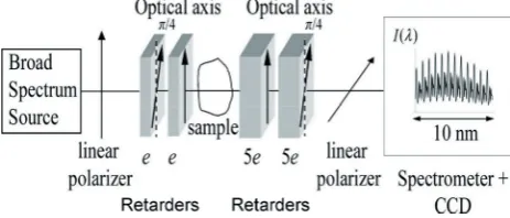
active element. The retrieval of the whole set of Mueller components requires the use of, at least, one polarizer plus two retarders for the polarization encoding, and two retarders plus one polarizer for its decoding. Figure 1 shows one among the possible configurations [6].
)LJSnapshot Mueller Matrix Polarimeter in the (e,e,5e,5e) configuration.
This configuration is denoted (e,e,5e,5e) by reference to the thicknesses of the different retarders, whose optical axes are oriented in the configuration (45°,0°,0°,45°) with the input polarizer and the output one set respectively at 0 and 90°. Let [P()] be the MM for a linear polarizer set at the angle , and [B(I,)] be the one for a retarder whereI and refer to the retardation and the fast axis orientation, respectively. In the Stokes-Mueller formalism, the action of the snapshot polarimeter on an input Stokes vector SJJGi
can be expressed as follows:
> @
2 . 5 , 4 . 5 , 0 . .
, 0 . , 4 . 0 .
o
i
S P B B M
B B P S
S I S I
I I S
ª¬ º ª¼ ¬ º ª¼ ¬ º¼
ª º ª º ª º
¬ ¼ ¬ ¼ ¬ ¼
G
G (2)
where [M] is the MM of the unknown sample. The intensity measured by the detector (spectrometer + CCD) is the first parameter of the output Stokes vector and can be written as:
00 02 20 22 01 21 0
02 22 0 12 0
11 0 10 12 0
11 0 12 0
22 33 0 21 0
20 22 0 21 0
22 33 0
32 ( ) 8 4 4 2 8 4 cos
4 2 cos 2 2 cos 3 4 cos 4 8 4 cos 5 4 cos 6 2 cos 7
cos 8 2 cos 9 4 2 cos 10 2 cos 11
cos 12 4
I m m m m m m f
m m f m f
m f m m f
m f m f
m m f m f
m m f m f
m m f
O O O O O O O O O O O O
03 23 0
13 0 13 0 23 32 0
13 0 30 32 0
31 0 23 32 0
2 sin 2
2 sin 3 2 sin 7 sin 8
2 sin 9 4 2 sin 10
2 sin 11 sin 12
m m f
m f m f m m f
m f m m f
m f m m f
O O O O O O O O O (3)
where mij (i, j = 0,…,3) are the coefficients of the Mueller matrix [M]. One should note that the mij coefficients are assumed to be wavelength-independent in the analysis window. The signal is composed, at the most, of 13 frequencies (from 0 to 12f0). The informative data are extracted in the Fourier domain, and the mij coefficients are proportional to the magnitudes of the Fourier peaks. Table 1 gives the relationships established between the magnitudes of the Fourier peaks and the mij coefficients in the case of the ideal configuration (e,e,5e,5e).
7DEOHRelationships between the magnitudes of the peaks (real and imaginary parts) and the Mueller coefficients (mij) in
the Fourier domain for the (e,e,5e,5e) configuration. Real Part Imaginary Part
Frequency Magnitude (x 64) Magnitude (x 64) 0 16m008m028m204m22 0
f0 8m014m21 0
2f0 4m022m22 4m032m23
3f0 2m12 2m13
4f0 4m11 0
5f0 8m104m12 0
6f0 4m11 0
7f0 2m12 2m13
8f0 m22m33 m23m32
9f0 2m21 2m31
10f0 4m202m22 4m302m32
11f0 2m21 2m31
12f0 m22m33 m23m32
These relationships can be expressed in matrix formalism as follows:
> @
.VG P XG (4)
where 0Re 1Re ... 12Re 1Im ... 12Im T
VG ¬ªV V V V V º¼ is a
25-dimension vector composed of the magnitudes of the
Fourier peaks and a
16-dimension vector composed of the Mueller coefficients. Thus, [P] is the 25 x 16 transformation matrix of the system and is only dependent on the thickness-configuration chosen for the retarders. The pseudo-inverse relationship expressed in Eq.(5) allows one to retrieve the Mueller coefficients from the measurement of the vector, V
>
00 01 ... 33@
TXG m m m
G :
> @ > @ > @
1( T. ) . T. .
XG P P P VG (5)
The necessary condition to build-up a snapshot polarimeter is the ability to inverse the transformation matrix. This is the case with the (e,e,5e,5e) configuration, but many other configurations also meet this requirement. As optimization of the thickness configuration was thoroughly studied in [7], only the main results will be recalled later.
2.2 Experimental setup
wavelength-independent. About the material in use for the retarders and their thicknesses, two conditions have to be met: i) the fundamental frequency, f0, must be high enough to get a sufficiently accurate Fourier-transformed signal, and ii) the highest frequency must be small enough to prevent the related peak magnitude from being dwindled by the detector response. These prerequisites drove us to employ retarders made of calcite (n(0) = 0.166) because the high birefringence of this material permits the use of rather thin plates, and thus, in this SMMP, the coding retarders are 2.08-mm-thick, whereas the decoding ones are 10.4-mm-thick. Under these conditions, a 6-oscillation signal is generated at the lowest frequency, f0, and 7 points are sampled per period at the 12f0-frequency, which largely meets the Nyquist criterion.
One should note that the source being partially coherent, the medium under study is imaged on a depolarizing medium, in turn imaged at the entrance of the detector.
2.3 Optimization of the configuration
As previously mentioned, several thickness configurations for the retarders permit the retrieval of every Mueller coefficient from the measurement of Fourier peaks. However, one of the main problems with snapshot techniques is the impact by random noise. But, it is nonsense to limit it through time-consuming repetitions of measurementsIt is, thus, worth choosing the configuration to be used from an established criterion about the propagation of random noise across MMs. Further to the thorough study reported in [7] and focused on the determination of the setup that guarantees the best noise immunity, let us introduce an additional matrix, [F], in relation (4) to take into account the cut-off frequency of the detection system:
> @> @
.VG F P XG ¬ ¼ª ºP X .G (6)
where [F] is a diagonal matrix and symbolizes a triangular window with fc as cut-off frequency. On condition to assume an additive white noise and no correlation between noise on the different Fourier peaks, one can use the EWV (Equally-Weighted Variance) criterion: this parameter is proportional to the variance of Mueller coefficients and calculated from the singular values, Pi, of the transformation matrix, ª º¬ ¼P :
16 16
2
1 1
1
EWV ( )i
i
i i
Var m
D
1 P
¦
¦
(7)Eq.(7) shows that the best configuration is the one where
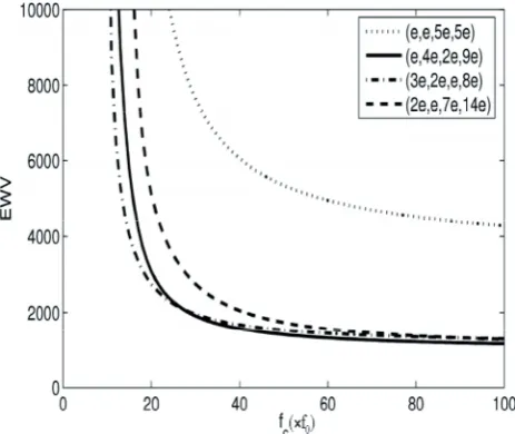
EWV value is the lowest. Calculations of EWV values through numerical simulations run on varying the thickness configuration denoted as (ke,le,me,ne), where
k,l,m,n are integer numbers, led to the identification of 4 configurations among the optimal ones (figure 2). Figure 2 highlights the existence of thickness-configurations better than the one in use in the
investigations reported here (e,e,5e,5e), which have been chosen before the drive of the optimization study. Depending on the cut-off frequency of the detection system, one can thus choose the most suited configuration for the retarder thicknesses.
)LJEWV versus fc for optimal configurations.
3 Calibration and stability
3.1 Systematic errors
With MM polarimeters, one needs to take into account systematic errors and to compensate for them. Two solutions are available: either the setup is described by a model, and then these errors must be well identified, or the setup is considered as a perfect unknown system, and the method developed by Compain [8] has to be used. In the present study, the simplicity of the elements at work in the setup together with the difficulties faced with the stability of the instrument led us to develop a model-dependent calibration procedure for the device. The setup retarders were thus considered as linear birefringent items with a retardance proportional to the wavelength (Eq.(1)). As the investigations reported in [9] were about the possible systematic errors liable to appear with a snapshot polarimeter, only the sources of imperfection and the way to compensate for them will be recalled below.
3.1.1 Setup-related errors
One of the main sources of systematic errors is the errors made on the thicknesses of the different retarders (e). For calcite plates, the uncertainty on thickness is around 0.01 mm, and thus the relationships between Fourier peaks and Mueller components are different from those given in Table 1 for the (e,e,5e,5e) configuration. As a consequence, an additional phase, Iw, has to be taken into account; its value will depend on the position of the signal I() in the analysis window. Moreover, it is worth underlining that the thicknesses of retarders 2, 3 and 4 are not strictly integer-multiple of the reference thickness, e.
(e,e+e2,5e+e3,5e+e4) and the phases associated to the thickness errors e2, e3, e4 by I2,I3,I4 given that Ip = (2nep)/0 (p = 2,3,4). The new relationships between the Fourier peaks and the Mueller coefficients are available in reference [9]. The knowledge of Iw,I2, I3 and I4 is a prerequisite toaccurate measurements. They are determined through use of two known media: i) vacuum, indeed its perfect knowledge allows accurate measurements of Iw, I2+I3 and I4, and ii) another medium to distinguish between I2 and I3; it can be a half-wave plate.
Another source of systematic errors is the errors made on the alignment of the optical axis of the retarders and on the azimuth of polarizers. The SMMP configuration under test assumes the alignment of optical elements as described in figure 1. But, as they cannot be strictly aligned in this ideal configuration, it is worth studying the overall impact by the misalignment errors on the four retarders, 1, 2, 3 and 4, and on the output polarizer. Because of the high number of optical elements at play, the development of the theoretical expressions relative to the misalignment-induced errors would be too complicated to gain insight. As shown in [9], thorough analyses of numerical simulations are a way to investigate the impact by these errors. It is worth noting that a combination of alignment errors may lead to an important error on the Mueller coefficients. To avoid this problem, a solution could be the inclusion of angular errors into the model, but these errors are very difficult to extract in the case of an SMMP. On condition that the misalignment of the optical elements is less than 0.1° thanks to the use, for example, of precise angular controllers, the accuracy on the Mueller coefficients should be less than 0.01.
The last important source of systematic error discussed here is the impact by the detector (spectrometer + CCD camera).
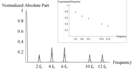
)LJTheoretical (black) and experimental (grey) absolute parts of the Fourier transform signal for vacuum. The inset
graph shows the experimental response of the detection calculated from vacuum signal.
Indeed, because of the numerical aperture of the optics, the detector has a limited bandwidth with regards to the quick variations of the intensity signals. This leads to a greater attenuation of Fourier peaks at higher frequencies. Figure 3 compares the theoretical and experimental magnitudes of Fourier peaks (absolute part) for vacuum and shows the strong reduction of the 12f0-frequency
peak, which is cut by more than twowith our setup. The response was measured through comparison of the heights of the Fourier peaks for theoretical and experimental signals from vacuum. The behavior displayed in the inset justifies the choice of a triangular window for the detection response used in Section 2.3.
3.1.2 Sample-related errors
One should be aware that, with SMMP, a non-uniform spectral response of the sample under study within the analysis window may induce an error on the measurement of the MM. Two sources of error have been identified: i) interference signal generated by multiple reflections into the medium under study and ii) evolution of Mueller coefficients with the wavelength.
The first source of error appears when the medium under study is, for example a wave-plate with no antireflection-coating. Indeed, multiple reflections on the two surfaces lead to an interference signal alike the one produced by a Fabry-Perot interferometer. Figure 4 presents the intensity spectrum, TFP(), of a wave-plate (about 1-mm-thick) set between crossed-polarizers. It is worth noting that the numerous oscillations would have been missing in the case of a plate with antireflection-coated faces. When such a medium is measured with an SMMP, the modulated signal, I() is overlaid by, TFP(), which generates systematic errors on the reconstructed MM.
)LJIntensity spectrum TFP() of a 1-mm-thick wave plate
set between crossed-polarizers
One should note that the frequency of the TFP() signal depends on the thickness of the medium under study. Typically, for a 10-nm-analysis window, the interference signal produced by a medium with an optical index of 1.5 and a thickness less than 1.5 mm generates systematic errors. A way to compensate for these errors is to know the TFP() signal shape from a measurement of the intensity spectrum of the medium under study set between crossed-polarizers. But, this implies to move the coding- and decoding-retarders. Another solution is to measure, with the SMMP, two signals denoted by IA( )O
( )
IA O and I//( )O , the device has to be upgraded by replacing the output linear polarizer with a Wollaston prism. Moreover, the “two-channel” setup permits a reduction of the retarder-associated errors, but also an enhancement of noise immunity because its EWV value is much lower than that of the single-channel SMMP (1142 against 3524). For these reasons, in our opinion the two-channel setup is liable to become a standard for snapshot measurements.
The second source of error appears in the case of strong mij variations with wavelength in the analysis window. Indeed, as the Fourier peaks are widened, their overlap generates deviations on the measured MMs. This consideration drove us to use a detection system with a narrow analysis window (10-nm wide). However, even in this spectral detection range, the polarimetric response of some media may evolve. It ensues that the evolutions of the mij components of the medium have to be compared with those of the coding retarders According to our previous study about the determination of the MM of a wave-plate [9], the evolution with wavelength of its phase difference in the analysis window must be less than 1% of that of the phase difference of the coding retarders. It is, thus, worth using thick retarders for the coding system to extend the validity range of the SMMP with still a good accuracy, even for a medium with wavelength-dependent mij coefficients.
3.2 Accuracy
To gain more insight into the degree of accuracy reached with the SMMP under test, experiments were carried out with two commercial media, i.e. a linear polarizer (ColorPol from Melles-Griot) and a quarter-wave plate (Melles-Griot). Figure 5 displays the Mueller coefficients versus the orientation angle of the polarizer, whereas figure 6 illustrates their evolution versus the fast axis orientation of the quarter-wave plate.
)LJTheoretical (continuous line) and experimental (square) Mueller coefficients versus the orientation of a
commercial linear polarizer
All of the Mueller components are normalized by m00. The acquisition time is 10 μs with 50 accumulations in order to reduce random noise. The experiment showed that, in both cases, the maximum error on Mueller coefficients was less than 0.03 (figures 5 and 6), which means that the accuracy on measurements is rather good.
)LJTheoretical (continuous line) and experimental (square) Mueller coefficients versus the orientation of the fast
axis of a commercial quarter-wave plate 3.3 Stability
Calcite retarders are sensitive to environmental changes, especially fluctuations in temperature. Their thickness is strongly affected by thermal expansion, and thus calibration values are no longer the same. As the thickness ratio between calcite plates is known, it would be worth making a simple measurement of temperature to recalculate the phases. This consideration drove us to investigate the relevance of using a model-dependent correction (linear thermal expansion). To gain more insight into the linearity of calcite plate length-expansion, a 5e-thickcalcite retarder was set between two crossed-polarizers.
)LJEvolution of the argument (phase) of the peak at 5f0
slow.Because of the nearly integer relationships between their respective thickness, if every calcite retarders undergoes the same temperature change, then only the value of Iw will vary. In [9], we showed that retrieving the value of Iw at any time is paramount. Whatever the medium under study, this method allows a direct measurement of Iw through, for example, the use of the arguments of 4f0 and 6f0 peaks. One should note that this implies that m11 is different from zero. Figure 8 illustrates how the Mueller coefficients are affected by a slow and slight change in temperature (0.2°C) and highlights the stabilization of every Mueller coefficient induced by the Iw correction. It also shows that, m03, m23 and m32are the most temperature-dependent: indeed, their variations with temperature are slow, but marked. On the other hand, the quick variations of mij are likely associated to random noise.
)LJEvolution of the Mueller coefficients of a no-sample measurement (vacuum) versus temperature over 15 minutes when the temperature changes were kept below 0.2°C. Solid curves represent Mueller coefficients with no correction, and
dashed curves show them after correction by Iw.
4 Time-resolved characterization of a
ferroelectric liquid crystal
Application of an electric field to ferroelectric liquid crystals (FLCs) is known to generate a fast response (about 100 μs). This led us to investigate the ability of the SMMP device to give a time-resolved description of fast switching in FLCs.To our knowledge, only two teams have performed time-resolved MM polarimetry on liquid crystals [11,12]. But, the polarimeters in use were sequential, so the MMs were reconstructed from various input and output polarization states and multiple synchronized acquisitions. Concerning the SMMP, its ability to acquire a full MM in a single shot should result in an enhancement of the signal-to-noise ratio. The chiral liquid crystal (LC) material under study is Felix 015/100, which has a birefringence around 0.16 in the visible/NIR. Two glass plates with transparent ITO electrodes and with a thin film of rubbed polyimide, produced by spin coating, are used to fabricate the cell. Its gap, obtained by spraying of spacers, is about 1.6 μm. The cell is then filled by capillary suction and the LC is confined between both plates in planar orientation which means that the LC molecules are parallel to the substrate. At room
temperature (25°C), this LC is in the smectic C* phase, where the molecular layers are perpendicular to the rubbing direction. The average orientation of molecule is specified by the unit vector , called the director (figure 9). The director is tilted by an angle with respect to the layer normal and in SC* bulk material, it rotates, forming a helical structure with the axis perpendicular to the layers. However, as the LC thickness is far below the helix pitch, and due to the planar anchoring conditions, the helical structure is suppressed so LC exhibits ferroelectricity properties. The spontaneous polarization,
nG
S
P JJG
, lies in the smectic layers and is perpendicular to the director. This structure is called SSFLC (Surface-Stabilized Ferroelectric Liquid Crystal) [13]. Application of an alternative electric field, , to this cell (figure 9) makes
E JG
S
P JJG
aligns with EJG and the molecules move between two stable states (“up” and “down”). The experiments were made with the FLC cell set perpendicular to the incident light.
)LJSSFLC cell and representation of the director (nG) in an (x,y,z) coordinate system; FLC molecules are symbolized by rigid sticks. The spontaneous polarization Ps is perpendicular to
the director, and tangential to the circle of intersection of the cone with the boundary plane of the layer.
4.1 Decomposition parameters
Liquid crystal molecules have a birefringent action on the incident light, and thus are well suited to polarimetric measurements. The parameters issued from experimental Mueller Matrices (M) were extracted by the Lu and Chipman decomposition [14], which consists in assuming that the medium under study is composed successively of a diattenuator, MD, a retarder, MR, and a depolarizer, M, so that M M M M' R D. For a FLC cell in normal
retardance, R, is linked to the angle, , by the following relationships:
0
2 n( )d
R S F
O
'
> @
> @
2 2 2 2
( ) e o
o
e o
n n
n n
n Cos n Sin
F
F F
'
(8)
where no is the ordinary index of the FLC, and ne is the extraordinary one. As R gives insight into the director position in the (Oy,Oz) plane, the knowledge of app and is sufficient to describe in a 3-D system on condition to assume a homogeneous distribution of the latter within the light beam. The last two parameters characterize the homogeneity of the director distribution. The ellipticity of the FLC cell-associated retarder appears when the distribution of the director orientation is non-homogeneous in the O
n G
z direction (twist). Indeed, if one considers a succession, in the Oz direction, of thin layers of thickness, , composed of molecules with an orientation, i, the resulting MM is MZ
MR( ,[ \i), where MR is the MM of a linear retarder of thickness, , and fast axis orientation, i. If i is varying across the total thickness, d, Mz will be an elliptic retarder. Ellipticity gives thus insight into the homogeneity of the director orientation along the cell thickness. The depolarization index, PD, is equal to 1 for an elliptic retarder. If one now considers, within the light beam (500μm), multiple areas with different orientation, i, the resulting MM is Mxy¦
M dR( ,\i). If i is varying within the (Ox,Oy) plane, PD associated to Mxy will decrease. One should note that this statement is valid because the FLC cell was imaged on a depolarizing medium, in turn imaged on the entrance of the detection system. The depolarization index is thus expected to evidence the presence of domains with different apparent angles at the beam scale.A key-asset of this method is the simultaneous extraction of all of the above parameters. It is the warrant of a good correlation between them, conversely to the case where several experiments are needed since they generate additional noise [11]. The technique described here is worth being used because of its non-invasivity, simplicity and good precision.
4.2 Experimental results
A square voltage between r 15 V at 30 Hz was applied to the FLC cell to investigate the dynamics of switching between the up and the down states. But the great difference between the CCD refreshment time and the duration of switching (| 1 ms vs | 100 μs) hindered its measurement over a single period. This drove us to synchronize the detection with the applied voltage; then, the acquisition was progressively delayed of the same time-increment to reconstruct the transition. Each MM was measured with a gate aperture of 5 μs and 25 accumulations. A total of 50 points were acquired with an increment of 6 μs. Figure 10 illustrates the time evolution of the four parameters under study.
)LJEvolution of the decomposition parameters, (R(t), R(t), PD(t), R(t)), throughout the “up”/“down” transition
The rotational viscosity, , of the liquid crystal is determined through extraction of the switching duration from R(t). Indeed, in the simplest theoretical model, the director behavior over the transition is described by
.I/t = PS.E.Sin[I], where I is the angle between the applied electric field, , and the spontaneous polarization,
E JG
S
P JJG
[16]. The transition rise-time tudis given by the interval between, for example, 10 and 90%. In this study, the spontaneous polarization value was given by
PS = 33 nC/cm2, the applied voltage was set at
E 10 V/μm and the measured rise-time was tud 70 μs. From the solution of the above equation expressed in [16], the relation tud K/(1, 32. . )P ES led to 0.175 Pa.s for the rotational viscosity. However, this simple relation gives a poor account of the true dynamic behavior since it fails to give a good fit of the experimental curve when only the ferroelectric torque is taken into account. A more elaborated model of the FLC switching dynamics will be presented and tested against experimental data elsewhere.
The minimum observed on the plot of R(t) (figure 10) corresponds to the lowest value of the angle, (see Eq.(8)). It indicates that, over the transition, the molecules get out of the cell plane for a while. Indeed, according to the theory, in FLC cells the molecules switch around a cone.
One should also note that PD is equal to 1 (uniform state) in the up and down states. The short minimum ( 0.900) means that, within the light beam, the various molecules switch from the up to down states at different times (dispersion of switching starts). However, a domain propagation-induced switching would have strongly lowered depolarization value ( 0.650).
According to figure 10, R is close to 0° in the up and down states, which means that the director distribution is almost homogeneous in the Oz direction despite a small twist, likely located near the surfaces due to the anchoring strengths. The change in R sign indicates a change in the direction of twist. Analysis of R behavior at the transition is more complex because of the non homogeneity of the director distribution in the (Ox,Oy) plane. On-going researches are focused on the development of a more detailed model of the director distribution within the cell to further quantify ellipticity and depolarization.
experimental angles, and app, linked to the director coordinates (x,y,z) by the following relations:
> @
> @
> @
app
app
x rSin Sin
y rSin Cos
z rCos
F T
F T
F
ª º
¬ ¼
ª
¬ º¼ (9)
where r is the size of the rigid stick that symbolizes the molecules. Figure 11 illustrates the trajectory followed by the molecules when they switch from the up to down states for two different positions of the light beam within the cell. One should note changes (from a cone to a deformed ellipse) in the shape of the different trajectories. This finding suggests the existence of different layer structures within the cell. The authors are currently trying to give more thorough interpretations of these results, which will be published elsewhere.
)LJRepresentation of the director end in the (Ox,Oz)
plane during the up/down transition for two positions of the beam within the cell. The trajectory showed in the left is calculated from the parameters represented in figure 10. This representation assumes a collective movement of the directors
(no depolarization). The associated error bars are for an uncertainty of 0.5°on the retardance value; r is normalized to 1.
5 Conclusion
This paper provided theoretical and experimental evidences of the relevance of using Snapshot Mueller matrix polarimetry by wavelength polarization coding. Indeed, as the polarimetric response is encoded in a single spectrum, the acquisition time of a full Mueller matrix only depends on the temporal achievement of the CCD camera used for the detection, and thus can be very short. The different sources of errors associated with the device were recalled as well as the ways to compensate for them. To enhance measurement accuracy, an optimization procedure was proposed: it consisted in choosing the best thickness-configuration for the retarders and upgrading the device through the two-channel setup. Moreover, methods were proposed to take into account the impact by temperature changes on the SMMP stability. At last, this setup was used to investigate fast switching of a ferroelectric liquid crystal by time-resolved Mueller matrix polarimetry. These experiments led to the description of the trajectory followed by the molecule director over electric field-induced transitions. They also brought additional information about the collective motions of the molecules. The SMMP technique is expected to open the way to new investigations on polarization phenomena made possible by its snapshot property.
References
1. E. Garcia-Caurel, A. De Martino, B. Drévillon, Thin Solid Films, , 120-123 (2004)
2. B. Laude-Boulesteix, A. De Martino, B. Drévillon, and L. Schwartz, Appl. Opt. , 2824-2832 (2004) 3. B.H. Ibrahim, S. Ben Hatit and A. De Martino, Appl.
Opt. , 5025-5034 (2009)
4. K. Oka and T. Kato, Opt. Lett. , 1475-1477 (1999) 5. N. Hagen, K. Oka, and E. L. Dereniak, Opt. Lett. ,
2100-2102 (2007)
6. M. Dubreuil, S. Rivet, B. Le Jeune, and J. Cariou, Opt. Express , 13660-13668 (2007)
7. P. Lemaillet, S. Rivet, and B. Le Jeune, Opt. Lett. , 144-146 (2008)
8. E. Compain, S. Poirier and B. Drévillon, Appl. Opt.
, 34903502 (1999)
9. M. Dubreuil, S. Rivet, B. Le Jeune, and J. Cariou, Appl. Opt. , 1135-1142 (2009)
10. M. Dubreuil, S.Rivet, B. Le Jeune and J.Cariou, Appl. Opt. , 6501-6505 (2009)
11. I.Dahl, Meas.Sci.Technol. , 1938-1948 (2001) 12. A. Lizana, I. Moreno, C. Iemmi, A. Márquez, J.
Campos, and M. J. Yzuel, Appl. Opt. , 4267-4274 (2008)
13. N.A. Clark and S.T. Lagerwall, Appl. Phys. Lett. , 899-901 (1980)
14. S-Y.Lu and R.A.Chipman, J. Opt. Soc. Am. A , 1106-1113 (1996)
15. F.Boulvert, G.Le Brun, B.Le Jeune, J.Cariou, L.Martin, Opt. Comm. , 692-704 (2009)
16. M.A. Handschy and N.A. Clark, Appl. Phys. Lett.