United Kingdom ISSN 2348 0386 Vol. VII, Issue 6, June 2019
Licensed under Creative Common Page 543
http://ijecm.co.uk/
MODELING AND FORECASTING THE PROCESS OF
PRODUCING WINE USING ECONOMETRIC PACKAGE EVIEWS
Sapaev Dilshod Khushnudovich
Applicant for PhD degree, Tashkent chemical-technological Institute, Uzbekistan [email protected]
Abstract
Modeling and forecasting of the manufacturing process becomes more and more actual.
The article proposes a method of using Eviews package for modeling and forecasting the
process of producing wine in the economic development of developing countries (the
Republic of Uzbekistan). The results of the study showed acceptability of the proposed
model for the development of the strategy for the develop ment of the viticulture-wine-making
branch.
Keywords: Modeling, Forecasting, Econometrics, Uzbekistan
INTRODUCTION
Economic and mathematical modeling is an integral part of any research in the field of defining a model of an economic development strategy. The development of mathematical analysis, operations research, probability theory and mathematical statistics contributed to the formation of various kinds of approaches to the study of issues of modeling the cluster development of the industry (Dennis et al, n.d.).
Licensed under Creative Common Page 544 The scientific literature describes the development of a number of specialized packages designed to build adequate econometric models. One of them is the EVIEWS package. The Eviews package allows regression estimation not only by the least squares method, but also by maximum likelihood methods, weighted and nonlinear least squares methods, it is enough to simply type the name of the method on the command line when estimating the model coefficients (Christopher and Robert, 1992).
But in the literature, it is difficult to find the use of the EVIEWS package based on statistical data of a certain sector of the economy. The use of this package in order to develop a model for forecasting and designing strategic development of viticulture and winemaking will help in determining competitive grape varieties, taking into account the influence of production factors, etc.
Complex composition of grapes, availability of various ways of their processing, quality control of the finished products, give the possibility to predict the type and name of finished products, their properties, corresponding to quality and features of each grape variety. In order to simplify predicting, we have divided all grape varieties into V Groups. The division took place based on the quality of the wine, produced from given grape variety and its characteristics.
METHODOLOGY
The methodology for compiling industry modeling is the subject of research and development of research organizations and companies that produce software packages in the field of economics. However, the techniques used in practice are often insufficient to obtain a comprehensive picture of the future strategy of an enterprise. This is due to the narrow specialization of existing systems, with the lack of support for business planning methods based on economic-mathematical methods and models.
Under the methodology of creating a model of the production process is understood a set of ways in which objects of an industry cluster are represented as a model. Any technique includes three main components:
- theoretical base;
-description of the steps necessary to obtain a given result;
- recommendations for use methods separately and as part of a group.
Licensed under Creative Common Page 545
RESULTS AND DISCUSSIONS
In the conditions of market economy, forecasting is the key of successful development of business and industry. Adoption of any strategic management decision requires foresight for the development of the economic situation. To do this, we use statistical methods of forecasting, using time series, taking into account past and current regularities of the industry development.
The time series is a set of numbers, attached to the serial, usually equidistant time points. Data on release or consumption of various goods within certain time are time series. Numbers that make up series and are resulting from observation of some process, are called elements, and the interval between observations –sampling time (Shodiev et al, 1999). Series elements are numbered according to the number of the timepoint to which this element belongs
(i.e. designated as (Y1, Y2, ...,Yn)).
Time series includes information about features and regularities of the forecasting process, and statistical analysis is used to assess characteristics of the process in the future. The task of forecasting come down to obtaining estimates of series values at some period in the
future, that is, to obtaining value Yp(t), t = N + 1, N+2, ... . Using extrapolation methods, we
proceeded from the assumption of maintaining regularities of the past development for the forecasting period. In many cases, when developing real-time forecast (up to one year) and short-term (up to 2 years) forecast, these assumptions are true.
The forecast is calculated for two stages. At the first stage- formal-using statistical methods, regularity of the past development is found, extrapolated for some period in the future.
At the second stage – correction of obtained forecast is performed, taking into account results of conceptual analysis of the current state.
Statistical research methods proceed from assumptions about possibility of presenting levels of time series as a sum of several components, reflecting the regularity and randomness of the development, particularly as the sum of four components:
Y(t) = f(t) + S(t) + U(t) + E(t), (1)
Where,
Y(t) – trend (long-term tendency) of development; S (t) – seasonal component;
U (t) – cyclical component;
Е (t) – residual component.
Licensed under Creative Common Page 546 For time series analysis, graphics methods are applied. As tabular presentation of the time series and descriptive characteristics often do not allow understanding the process nature, and on time series chart, it is possible to make certain conclusions, which can be checked then, using calculations.
For modeling and forecasting the process of producing wine from grapes, modern econometric package Eviews is used. It is a modern statistical package, "intended" for time-series analysis, and it presents wide opportunities when analyzing the data, presented in the
form of time series (Kasimov 2017). For building multi-factor econometric model, logarithmic
initial data are given in table 1.
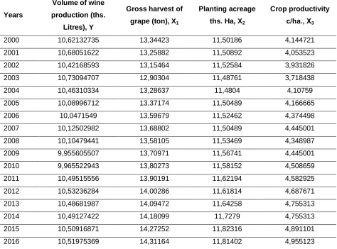
Table 1 Logarithmic initial data
Years
Volume of wine
production (ths.
Litres), Y
Gross harvest of
grape (ton), X1
Planting acreage
ths. Ha, X2
Crop productivity c/hа., X3
2000 10,62132735 13,34423 11,50186 4,144721
2001 10,68051622 13,25882 11,50892 4,053523
2002 10,42168593 13,15464 11,52584 3,931826
2003 10,73094707 12,90304 11,48761 3,718438
2004 10,46310334 13,28637 11,4804 4,10759
2005 10,08996712 13,37174 11,50489 4,166665
2006 10,0471549 13,59679 11,52462 4,374498
2007 10,12502982 13,68802 11,50489 4,445001
2008 10,10479441 13,58105 11,53469 4,348987
2009 9,955605507 13,70971 11,56741 4,445001
2010 9,965522943 13,80273 11,58152 4,508659
2011 10,49515556 13,90191 11,62194 4,582925
2012 10,53236284 14,00286 11,61814 4,687671
2013 10,48681987 14,09472 11,64258 4,755313
2014 10,49127422 14,18099 11,7279 4,755313
2015 10,50916871 14,27252 11,82316 4,891101
2016 10,51975369 14,31164 11,81402 4,955123
Source: Initial data got from annual report of Agency of development vine and wine industry and investigations of FAO published in internet
Licensed under Creative Common Page 547 Table 2 Results of descriptive statistics
Name of values Y X1 X2 X3
Mean 10.36707 13.67422 11.58649 4.404256
Median 10.48682 13.68802 11.53469 4.445001
Maximum 10.73095 14.31164 11.82316 4.955123
Minimum 9.955606 12.90304 11.48040 3.718438
Std. Dev. 0.257579 0.416718 0.109341 0.348724
Skewness -0.405278 -0.059383 1.142734 -0.196781
Kurtosis 1.705656 1.991577 3.095753 2.190794
Jarque-Bera 1.652065 0.730308 3.706377 0.573542
Probability 0.437783 0.694090 0.156737 0.750684
Sum 176.2402 232.4618 196.9704 74.87235
Sum Sq. Dev. 1.061553 2.778460 0.191289 1.945730
Observations 17 17 17 17
Table 2 identifies mean value (mean), median values (median), standard deviations (std.Dev.), minimum and maximum values (max, min) of variables.
0.0 0.5 1.0 1.5 2.0 2.5 3.0
9.6 9.8 10.0 10.2 10.4 10.6 10.8 11.0 11.2
D
e
n
s
it
y
Y
0.0 0.2 0.4 0.6 0.8 1.0
12.4 12.8 13.2 13.6 14.0 14.4 14.8
D
e
n
s
it
y
X1
0 2 4 6 8 10
11.3 11.4 11.5 11.6 11.7 11.8 11.9 12.0
D
e
n
s
it
y
X2
0.0 0.2 0.4 0.6 0.8 1.0 1.2
3.2 3.4 3.6 3.8 4.0 4.2 4.4 4.6 4.8 5.0 5.2 5.4
Histogram Kernel Normal
D
e
n
s
it
y
X3
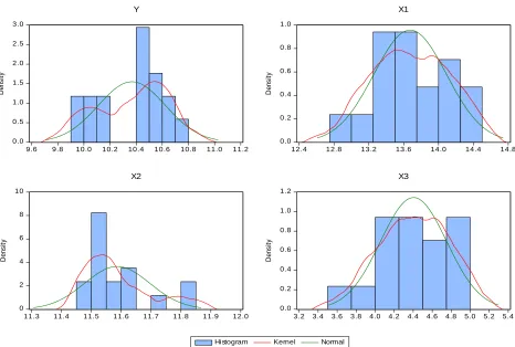
Licensed under Creative Common Page 548 Visual analysis of time series chart (histogram) allowed making conclusions:
• existence of trend and its nature;
• presence of seasonal and cyclical components;
• degrees of smoothness or intermittence of changes of series consecutive values after removal of trend.
As figure 1 shows, variables Х1 and Х3 correspond to normal distribution law. Variable Y has
left-handed bias, and variable Х2 has right-handed bias. Because values of asymmetry
coefficients adopt negative and positive values.
To verify the relationship between variables, coefficients of partial and pair correlation are calculated (table. 3).
Table 3 Coefficients of partial and pair correlation Covariance Analysis: Ordinary
Date: 11/17/18 Time: 11:21 Sample: 2000 2016
Included observations: 17
Correlation t-Statistic
Y X1 X2 X3
Y 1.000000
X1 -0.068559 1.000000
X2 0.205707 0.879621 1.000000
X3 -0.104236 0.996627 0.855261 1.000000
The next step is the analysis of partial correlation coefficient.
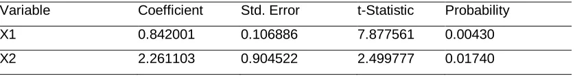
Table 4 Calculation of multi-factor econometric model Dependent Variable: Y
Method: Least Squares Date: 11/17/18 Time: 11:28 Sample: 2000 2016
Included observations: 17
Variable Coefficient Std. Error t-Statistic Probability
X1 0.842001 0.106886 7.877561 0.00430
Licensed under Creative Common Page 549
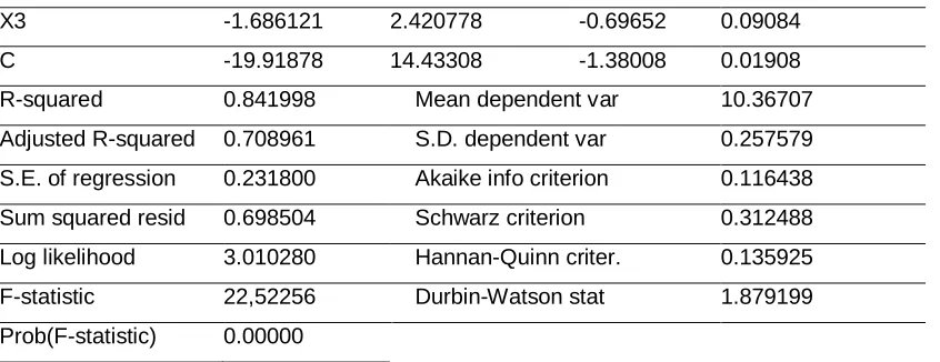
X3 -1.686121 2.420778 -0.69652 0.09084
C -19.91878 14.43308 -1.38008 0.01908
R-squared 0.841998 Mean dependent var 10.36707 Adjusted R-squared 0.708961 S.D. dependent var 0.257579 S.E. of regression 0.231800 Akaike info criterion 0.116438 Sum squared resid 0.698504 Schwarz criterion 0.312488 Log likelihood 3.010280 Hannan-Quinn criter. 0.135925 F-statistic 22,52256 Durbin-Watson stat 1.879199 Prob(F-statistic) 0.00000
Then multi-factor econometric model is built, which looks as follows:
3 2
1
2
,
261
1
,
686
842
,
0
92
,
19
ˆ
X
X
X
Y
Analysis of the obtained multifactor model has shown that:
- 1 ton increase in gross harvest of grapes (x1) will lead to increase in volume of wine production
on average by 0.842 tons;
- 1 ha increase in the planting acreage of grapes will lead to increase in volume of wine production on average by 2.261 tons;
- 1 centner/ha decrease in crop productivity of grapes will lead to reduction of wine production volume on average by 1.686 tons.
Verification of statistical significance of obtained multi-factor model was conducted, using coefficient of determination.
Estimated value of the coefficient of determination is
0
,
8419
2
R
. This shows that the volumeof wine production (Y) by 84.19 percent depends on factors, included in the model, i.e.:
- gross harvest of grapes (Х1);
- planting acreage of grapes (Х2);
- crop productivity of grapes (Х3).
The rest 15.81 per cent (100-84,19) is the influence of unaccounted factors.
To determine adequacy of the received model, F value of Fisher statistics is used. If Fest.>Ftab.,
obtained model is adequate for the studied process. Since Fest.=22,52, and Ftab.=3,16, it can be
said that obtained model is adequate.
Check of reliability of multi-factor model coefficients showed the use of t-statistic of Student. If
test.>ttab., obtained coefficients of multi-factor model are reliable. Since tx1=7,877, tx2=2,499, tx3
=-0,696, and ttab.=2,43, we can say that factors Х1 and Х2 are reliable. Factor Х3 is considered
unreliable.
Licensed under Creative Common Page 550 Check of autocorrelation of Y series remainders was based on the use of Durbin-Watson statistics. If estimated value of Durbin Watson statistics adopt value between 2 and 4, in the series remainder, there is no autocorrelation. In our calculation, Durbin-Watson statistic takes value 1.879199. This shows that in the studied series there is no autocorrelation.
Based on obtained multi-factor model`, volume of wine production in the Republic of Uzbekistan is forecasted.
Table 5 Forecasted value of wine production volume and factors, affecting it, for 2018-2021 Years Volume of wine
production (ths. litres)
Gross harvest of grapes (ton)
Planting acreage ths. ha
Crop productivity c/hа.
2018* 37808,1 1894880 130190,5 155,9
2019* 37841,7 2048688 132691,2 166,3
2020* 37875,4 2214980 135240,0 177,3
2021* 37909,1 2394771 137837,7 189,1
On the basis of forecasted values of multi-factor models, appropriate graphics are built (figure 2–5).
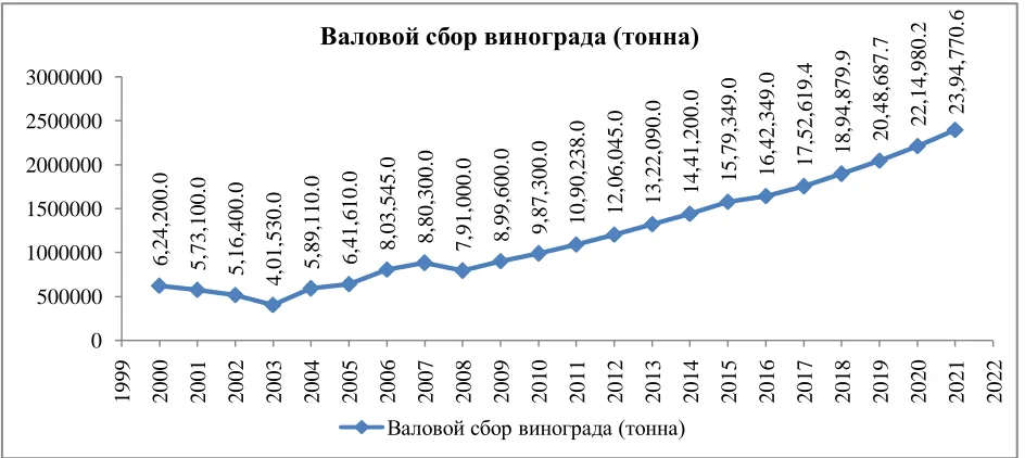
Figure 2 Forecast of bulk yield of grapes
6, 24, 200. 0 5, 73, 100. 0 5, 16, 400. 0 4, 01, 530. 0 5, 89, 110. 0 6, 41, 610. 0 8, 03, 545 .0 8, 80, 300. 0 7, 91, 000 .0 8, 99, 600. 0 9, 87, 300. 0 10, 90, 238. 0 12, 06, 045. 0 13, 22, 090. 0 14, 41, 200. 0 15, 79, 349. 0 16, 42, 349. 0 17, 52, 619 .4 18, 94, 879. 9 20, 48, 687. 7 22, 14, 980. 2 23, 94, 770. 6 0 500000 1000000 1500000 2000000 2500000 3000000
1999 2000 2001 2002 2003 2004 2005 2006 2007 2008 2009 2010 2011 2012 2013 2014 2015 2016 2017 2018 2019 2020 2021 2022
Валовой сбор винограда (тонна)
Licensed under Creative Common Page 551 Figure 3 Forecast of grapes planting acreage
Figure 4 Forecast of grapes crop productivity
98, 900. 0 99, 600. 0 1, 01, 300. 0 97, 500 .0 96, 800 .0 99, 200 .0 1, 01, 176. 0 99, 200. 0 1, 02, 200. 0 1, 05, 600. 0 1, 07, 100. 0 1, 11, 518. 0 1, 11, 095. 0 1, 13, 843. 0 1, 23, 983. 0 1, 36, 374. 0 1, 35, 134. 0 1, 27, 736. 9 1, 30, 190. 5 1, 32, 691. 2 1, 35, 240. 0 1, 37, 837. 7 80000 90000 100000 110000 120000 130000 140000 150000
1999 2000 2001 2002 2003 2004 2005 2006 2007 2008 2009 2010 2011 2012 2013 2014 2015 2016 2017 2018 2019 2020 2021 2022
Площадь посева тыс. га
Площадь посева тыс. га 63. 1 57. 6 51. 0 41. 2 60. 8 64. 5 79. 4 85. 2 77. 4 85. 2 90. 8 97. 8 108 .6 116. 2 116. 2 133 .1 141. 9 146. 1 155 .9 166. 3 177. 3 189. 1 0 20 40 60 80 100 120 140 160 180 2001999 2000 2001 2002 2003 2004 2005 2006 2007 2008 2009 2010 2011 2012 2013 2014 2015 2016 2017 2018 2019 2020 2021 2022
Урожайность ц/га
Licensed under Creative Common Page 552 Figure 5 Forecast of wine production volume
According to forecast calculations, continuous growth of grapes gross harvest due to increase in grapes planting acreage and crop productivity per hectare is observed, while the volume of wine production remains roughly at the same level.
CONCLUSION
Studies have shown that use of this model will allow improving the system of modeling and forecasting of the production process of the viticulture-wine-making branch in the Republic of Uzbekistan, this, in turn, will contribute to formation of strategy of industry cluster development. The forecast for various planning intervals in the wine industry is the basis for calculating and adjusting the output. In order to achieve higher results, the tasks assigned should be understood comprehensively and carried out in accordance with the established structure of objectives.
The paper discusses the factors affecting the efficiency of the production process, in the performance of which the selling price of the finished product will meet the predicted value. Conducted study is not enough for exploration of the entire industry, therefore it is preferable to develop econometric models to determine wines quality on the basis of characteristics of grape varieties. 41, 000. 0 43, 500 .0 33, 580 .0 45, 750. 0 35, 000. 0 24, 100. 0 23, 090. 0 24, 960. 0 24, 460. 0 21, 070. 0 21, 280. 0 36, 140. 0 37, 510. 0 35, 840. 0 36, 000 .0 36, 650 .0 37, 040. 0 37, 774. 5 37, 808. 1 37, 841. 7 37, 875. 4 37, 909. 1 20000 25000 30000 35000 40000 45000 50000
1999 2000 2001 2002 2003 2004 2005 2006 2007 2008 2009 2010 2011 2012 2013 2014 2015 2016 2017 2018 2019 2020 2021 2022
Объем производства вина (тыс. литров)
Licensed under Creative Common Page 553
REFERENCES
Christopher Winship and Robert D (1992). Mare, Models for Sample Selection Bias, Annual Review of Sociology, Vol. 18 (1992), pp. 327-350
Dennis E. Blumenfeld, Debra A. Elkins, and Jeffrey M. Alden (n.d.), Mathematics and Operations Research in Industry, https://www.maa.org/mathematics-and-operations-research-in-industry
Kasimov S.М. Sapaev D.Kh. (2017), Regional forecasting in the development of viticulture-wine-making branch of the Republic of Uzbekistan // 2 International Scientific Conference of promising developments of young scientists « Science of young-the future of Russia »: Collection of scientific articles. December 13-14, 2017 , Kursk, 2017. V. 1p. 182- 185