Betweenness versus Linerank

(1)

Betweenness versus Linerank

Balázs Kósa, Márton Balassi, Péter Englert, and Attila Kiss

Eötvös Loránd University, 1117 Budapest, Pázmány Péter sétány 1/C

{balhal,bamrabi,enpraai,kiss}@inf.elte.hu

Abstract. In our paper we compare two centrality measures of networks, between-ness and Linerank. Betweenbetween-ness is widely used, however, its computation is expen-sive for large networks. Calculating Linerank remains manageable even for graphs of billion nodes, it was offered as a substitute of betweenness in [12]. To the best of our knowledge the relationship between these measures has never been seriously examined. We calculate the Pearson’s and Spearman’s correlation coefficients for both node and edge variants of these measures. For edges the correlation tends to be rather low. Our tests with the Girvan-Newman algorithm [16] also underline that edge betweenness cannot be substituted with edge Linerank. The results for the node variants are more promising. The correlation coefficients are close to1. Notwith-standing, the practical application in which the robustness of social and web graphs is examined node betweenness still outperforms node Linerank. We also clarify how Linerank should be computed on undirected graphs.

Keywords: big data, networks, centrality measures, betweenness, Linerank.

1. Introduction

As part of the ever more important big data analysis [19], the study of network centrality measures offers unique challenges [10, 18]. In a network centrality measures indicate the importance, interestingness of the nodes and the edges and they play a crucial role in many solutions to practical problems e.g. who are the most influential opinion-shapers in a community, which web pages contain the most relevant information about a certain topic [17] or which nodes should be deleted from a network in order to make the system to fall to pieces [3].

In our paper we compare different centrality measures, namely node and edge be-tweenness with node and edge Linerank respectively from different aspects. First, the Pearson’s and Spearman’s correlation coefficients are calculated both on real world and generated graphs. It turns out that the correlation between node Linerank and betweenness is higher than0.9almost in all cases, whereas for the edge versions it ranges from0.2to 0.7. These results suggest that node Linerank is a very promising candidate for substitut-ing node betweenness, while this interchangeability is far more questionable for the edge variants. To further assess the applicability of Linerank we present the same correlation measures for approximates of betweenness, where instead of the_O(nm)runtime of we perform a sampling in_O(√nm)or as low as_O(log(n)m)runtime.

(2)

the Girvan-Newman algorithm. In our experiment instead of betweenness we calculated the Linerank value of the edges. In the comparison we used the same random benchmark graphs as in the calculation of the correlation coefficients. The results clearly show that the betweenness version significantly outperforms the Linerank version. On the one hand, this is not surprising since we have already observed that the correlation between these two measures is varying and it is never too strong. On the other hand, in their original paper Girvan and Newman tried three different variants of the betweenness measure and they found that the quality of the clusterings was not affected noticeably by the choice of the centrality measure. Our analysis reveals that this is no longer the case in the case of Linerank.

Secondly, we repeated the experiments of Boldi et al. in which they examined which nodes have the strongest impact in determining the structure of a network [3]. Or, in other words, which node-removal order influences this structure the most. They consid-ered several centrality measures including Pagerank, harmonic centrality and between-ness. They removed the nodes in decreasing order according to these measures. Contrast to the Girvan-Newman algorithm however, in this case the order of the removal was fixed in the first step, which means that the aforementioned values were not recalculated after each deletion. The authors reported that in several cases betweenness outperformed the rest of the candidates. In our research instead of taking into account several centrality measures we focused solely on node betweenness and Linerank. Unlike in the previous case the difference between the performance of these two measures was unnoticeable for the generated benchmark graphs. However, in the case of real world graph networks be-tweenness outperformed Linerank again. This indicates that in practice one should still be careful when node betweenness is to be substituted with node Linerank.

The paper is organized as follows. In Section 2 the related work is presented. In Sec-tion 3 the algorithm used for approximating betweenness and its expected behaviour is described. In Section 4 the computation of Linerank is explained in more detail. Next, in Section 5 the results of our experiments are delineated. In Section 5.1 the Pearson’s and Spearman’s correlation coefficients are calculated. Then, in Section 5.3 edge between-ness is compared to edge Linerank by using the Girvan-Newman algorithm. Afterwards, in Section 5.4 the node variants are considered in order to determine the node removal order in networks and then to assess the influence of these removal orders. Finally, in Section 6 we conclude by summarizing our work. This paper is an extended version of the paper of the same name published at ICCCI 2014 [1].1

2. Related Work

In [12] centrality measures are divided into three families. The first group is constituted by the degree related measures, the second group consists of the diameter related measures, while the third group contains the flow based measures. We focus on the last group in our paper. Here, flow refers to the amount of information that may pass through a node or an edge. The most important member of this group, betweenness centrality, was proposed

1_{This work was partially supported by the European Union and the European Social Fund through}

(3)

by Freeman2_{. For a given node}_{v, it measures the ratio of those shortest paths that go}

throughv. Formally,vbet ₌P

u,w

bu,v,w

bu,w , wherebu,wandbu,v,w respectively denote the

number of the shortest paths between nodesu,wand the number of those shortest paths from the previous ones that pass throughv. The definition of this measure on edges can be formulated in a similar way.

Unfortunately, the computation of the exact values of betweenness is prohibitively expensive for large networks. For the ’node-variant’ the best known algorithms work in time_O(nm), wherendenotes the number of nodes, while mthe number of edges in a graph [12]. For this reason several attempts have been made to estimate the value of betweenness by using a carefully selected sample. As an orthogonal direction in [12] a new flow based centrality measure, Linerank, was introduced whose computation remains practically manageable even for graphs of billion nodes. As its name suggests the defi-nition of Linerank was greatly inspired by Pagerank [17]. Roughly speaking, in the first step the original graph is transformed into the corresponding line graph on which the Pagerank values of the nodes are calculated. Since in a line graph the nodes represent the edges of the original graph by accomplishing the previous step one gains values mea-suring the importance of edges in a similar way as Pagerank measures the importance of nodes. However, we want to emphasize that in [12] this measure on edges has not been introduced, Linerank has been only defined on nodes. Our results below confirm that this was a wise decision indeed in the sense of the use case of substituting betweenness with Linerank. Nevertheless, in what follows we will refer to this measure as edge Linerank. In order to obtain a measure on nodes the previous scores of the incident edges of a node should be aggregated. The details will be given in Section 4.

Of the many approaches that exist for community detection, such as leader-driven community detection [20, 11] or mixed graph models [13], the Girvan-Newman commu-nity detection algorithm [16] is one of the most well-known. Here, edges are removed from the graph according to the decreasing order of their betweenness values. However, after the removal of the edge with the highest betweenness score the betweenness val-ues of the remaining edges should be recalculated in each step. Sooner or later the graph falls to pieces and the resulting components are to be considered as communities. Of course, later these clusters may also be broken into to pieces. The hierarchy of commu-nities is depicted by means of a dendrogram. Each level of this tree represents a possible clustering. In the last step the one with the highest modularity is chosen to be the final solution. In order to evaluate the performances of the betweenness and Linerank versions of the Girvan-Newman algorithm we applied normalized mutual information, since it is a widely used measure for testing the effectiveness of network clustering algorithms [8].

To generate random graphs, the model in [14] was used. This model generates graphs with communities, whose sizes vary according to a power law distribution with exponent β. The degree distribution is also assumed to be power law with exponentγ. Beside these parameters one can specify a mixing parameterµs.t. each node shares a fraction1−µof its edges with the nodes of its cluster and a fractionµwith the other nodes of the graph. The number of nodes is also given as a parameter.

2_{Strictly speaking, Anthonisse introduced this measure earlier than Freeman in a technical report,}

(4)

3. The Algorithm of Estimating Betweenness

The algorithm, which we have used in our comparisons [5], approximate the exact be-tweenness values by using a sample of size√nor as low aslog(n), wherendenotes the number of nodes in the graph. In the paper, where the state of the art method of computing the betweenness values is presented [4], the formula of the betweenness value of nodev is rewritten in the following way:

vbet=X

u,w

bu,v,w

bu,w

=X

u,w

δ(u, w, v) =X

u

δ(u, v), whereX

w

δ(u, w, v) =δ(u, v).

Here,δ(u, v)is called the one-sided dependency ofuonv. Basically, in [4] these one-sided dependencies are calculated for each nodeuby using a breadth-first search to find the shortest paths fromuand then applying a cunning bottom-up labelling strategy, which results the desired betweenness values. In the estimation of [5] only a subset of the nodes are selected to calculate the one-sided dependencies. The theoretical justification of the method is provided by a result of Hoeffding [9], who has proven that for independent, identically distributed random variablesX1, . . . , Xkwith0≤Xi≤M (0≤i≤k)and

an arbitraryξ≥0:

P

X1+. . .+Xk

k −E

X1+. . .+Xk

k

≥

ξ

≤e−2k(Mξ)

2 .

In our case, for a randomly selected nodepi

Xi(v) =

n

n₋1δ(pi, v)

is used as a single estimate. Setting

M = n

n−1(n−2), ξ=ε(n−2)

Hoeffding’s bound can be applied. Namely, since the expectation of estimate 1_k(X1(v) +

. . .+Xk(v))is equal to the betweenness value ofvHoeffding’s bound guarantees that

the error of the approximation is bounded from above byε(n−2)with probability at least

e−2k

ε(n−2)

n

n−1(n−2)

2

, which ise−2k(ε(n−1)

n )

2 [5].

In [5] several strategies for random selection had been compared, and it turned out that in overall the method of selecting the nodes based on the uniform distribution outperforms the rest of the strategies. Thus, in our paper we also implemented this version. In [7] it is stated thatk ∈ O(log(n))samples are sufficient for approximating closeness centrality. To benchmark our results with Linerank we measured the performance of betweenness and edge betweenness with both_O(log(n))and_O(√n)samples.

4. The Computation of Linerank

(5)

1

2

3

1

3

2

1

2

3 4

5

6

v

1 ₂

5 u

6

3 4

1 2

3 1

3 2

(a) (b) (c) (d)

(e)

(f)

(g)

. . .1

k. . .

1

k. . .

1

n

.. .

1

n

|{z}

P

= 1

1

n

.. .

1

n =

(h) u

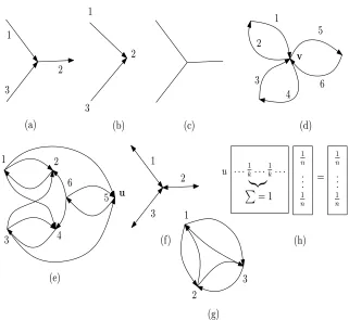
Fig. 1. (a) A graphGwith weights. (b)L(G). (c) An undirected graphH. (d)H˜. (e)

(6)

original graph is represented by a node. LetGbe a directed graph and lete1= (u1, v1),

e2 = (u2, v2)be edges ofG. InL(G)there is an edge from the node representinge1to

the node representinge2, if and only ifv1coincides withu2, i.e., the target node ofe1is

the same as the source node ofe2. An example can be seen in Fig. 1. (a) and (b).

On the line graph a random walker at the current step either moves to a neighbouring node with probabilityβ, or jumps to a random node with probability1−β. If the walker moves to a neighbouring node, then she decides among the candidates according to the weights of the joining edges. We seek the stationary probabilities of this random walk. Or, to put in other words Pagerank is to be computed on the line graph. However, the size of the line graph can be much larger than that of the original graph which may render the explicit construction of the adjacency matrix unfeasible. Therefore, in [12] this adjacency matrix is decomposed into two sparse matrices by means of which the stationary proba-bilities can be computed efficiently. In the last step for each node of the original graph the scores of its incident edges are aggregated.

The original paper does not detail how Linerank should be calculated over undirected graphs. It is tempting to substitute each undirected edge with two oppositely directed edges. However, this approach would result in completely useless Linerank values. To be specific for graphGdenoteG˜ the result of the previous construction. Then the following statement can be proven.

Proposition 1 Let Gbe an undirected graph. For each nodeuofL( ˜G) the outdegree

of each of the in-neighbours ofuis the same as the indegree ofu. (An in-neighbour is

defined to be the source node of an ingoing edge ofu.)

Proof. First, note that if the indegree of a nodevinG˜isk, then the outdegree ofvis also k, which is a straightforward consequence of the definition ofG. The statement obviously˜ follows from this observation, since in this case the indegree of the representative of an outgoing edge – denote itu– ofvinL( ˜G)is alsok. What is more, the outdegree of each of the in-neighbours ofuis alsokas they correspond to the ingoing edges ofv. Consider an example in Fig. 1. (c)-(e).

Corollary 1 For an arbitrary undirected, uniformly weighted graph G the stationary

probabilities – Pagerank values – are the same for each node ofL( ˜G).

Proof. (Sketch.) Consider the matrix used in the computation of the Pagerank values of

the nodes ofL( ˜G). From Proposition 1 it follows that the values of a tuple of this matrix are either0’s or1

k’s, wherekis the indegree of the represented node by this tuple. What is

more the sum of these 1_k values is equal to1. Hence, when the product of this matrix and vector(1

n. . . 1

n)is calculated at the first step of the computation, then the result is equal

to the same(1 n. . .

1

n)vector (Fig. 1. (h)), thus the computation terminates resulting the

same Pagerank values (stationary probabilites) for all nodes.

(7)

5. Experiments

5.1. The Correlation between Linerank and Betweenness

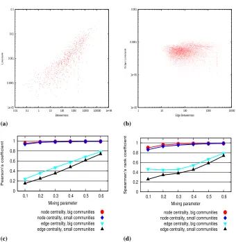
As a first step in our investigation we calculated the betweenness and Linerank values of the nodes and the edges of real world graphs. In all cases the scatter plots suggested a strong correlation between the node Linerank and betweenness values, whereas for the edge variants the relationship remained somewhat blurred. As a typical example in Fig-ure 2 (a) and (b) we have included the plots belonging to the polblogs dataset [2], a directed network of hyperlinks between weblogs on US politics recorded in 2005 with 1490nodes and19090edges. Beside the aforementioned real world graphs we also con-ducted the same experiment on random graphs described in the introduction. Owing to the costly computation of the exact betweenness values we used graphs of rather smaller sizes, namely with1000and5000nodes. Theγexponent of the power law distribution of the degrees was set to2, while theβ exponent of the power law distribution of the sizes of the clusters was chosen to be1. We further distinguished two cases. In the first case we worked with rather large clusters whose size ranged between20and100nodes, while in the second case this size ranged between10and50. The mixing parameter varied between0.1and0.6with steps of0.1. The plots revealed the same connection between the Linerank and betweenness values as in the case of the real world graphs.

Next, to quantify this relationship we calculated the Pearson’s and Spearman’s corre-lation coefficients of the two measures. For the polblogs dataset these values were high for the node variants of the centrality measures: Pearson’s:0.82Spearman’s:0.89; while for the edge variants the correlation turned out to be much weaker: Pearson’s:0.15 Spear-man’s:0.26. In the case of the random benchmark graphs we generated10graphs for every parameter settings and took the average of the results. In Figure 2 (c) and (d) the relevant diagrams can be found for graphs with5000nodes. The curves for the graphs with1000nodes look like almost exactly the same.

Interestingly, both for the node and edge variants the correlation between the centrality measures increases as the boundaries among the clusters becomes blurred. However, for the node versions it is very high in all cases and as the value of the mixing parameter grows the correlation approaches to1, whereas for the edge variants the correlation becomes higher only when the clusters literally disappear from the graph.

5.2. Correlation between Betweenness and its approximations

Another possible route for providing feasible approximations of the algorithms described in Subsection 5.3 and 5.4 would be to approximate the measure of betweenness itself instead of substituting it as suggested in [5]. Compared to [5] we use different indicators to assess the results, a namely Spearman’s and Pearson’ correlation coefficients as in Section 5.1.

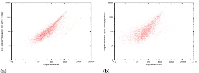
To demonstrate the efficiency of the approximation we have plotted the results for the polblogs dataset [2], that has also been used for the experiments in Subsection 5.1. The correlation coefficents were measured as presented in Table 1.

The node betweenness approximating algorithms performed exceptionally well from √

(8)

1e−05 0.0001 0.001 0.01 0.1

0.01 0.1 1 10 100 1000 10000 100000 1e+06

Linerank

Betweenness

(a)

1e−06 1e−05 0.0001 0.001

1 10 100 1000 10000

Edge Linerank

Edge Betweenness

(b)

0 0.2 0.4 0.6 0.8 1

0.1 0.2 0.3 0.4 0.5 0.6

Pearson’s coefficient

Mixing parameter

node centrality, big communities node centrality, small communities edge centrality, big communities edge centrality, small communities

(c)

0 0.2 0.4 0.6 0.8 1

0.1 0.2 0.3 0.4 0.5 0.6

Spearman’s rank coefficient

Mixing parameter

(d)

Fig. 2. (a) Node betweenness and Linerank values for the polblogs dataset. (b) Edge betweenness and Linerank for the same dataset. (c) Pearson’s correlation coefficients for the benchmark graphs with 5000 nodes. (d) Spearman’s correlation coefficients for the same set of benchmark graphs.

Table 1. Correlation for approximating betweenness values on the polblogs dataset Coeff. Node appr.,√

n Node appr.,log(n) Edge appr.,√

n Edge appr.,log(n)

Pearson 0.87 0.75 0.34 0.16

(9)

0.01 0.1 1 10 100 1000 10000 100000 1e+06

Betweenness approx. from sqrt(n) vertices

Betweenness

(a)

0.1 1 10 100 1000 10000 100000 1e+06

0.01 0.1 1 10 100 1000 10000 100000 1e+06

Betweenness approx. from log(n) vertices

Betweenness

(b)

Fig. 3. (a) Node betweenness and Node betweenness approximation from√nvalues for

the polblogs dataset. (b) Node betweenness and Node betweenness approximation from log(n)values for the for the same dataset.

1 10 100 1000 10000

0.1 1 10 100 1000 10000 100000

Edge Betweenness approx. from sqrt(n) vertices

Edge Betweenness

(a)

1 10 100 1000 10000

0.1 1 10 100 1000 10000 100000 1e+06

Edge Betweenness approx. from log(n) vertices

Edge Betweenness

(b)

Fig. 4. (a) Edge betweenness and Edge betweenness approximation from√nvalues for

(10)

lower runtime than the one usinglog(n)sample vertices. The edge variant of the mea-sure is significantly less promising. The approximation itself is not on par with its node counterpart, but still outperforms edge Linerank in both cases.

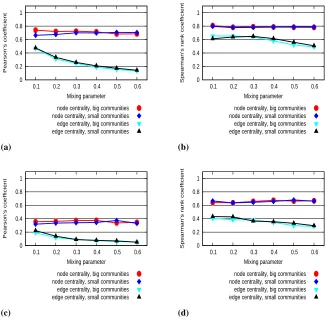
We have also conducted experiments on the benchmark graph dataset described in Subsection 5.1. The baseline for the result were the results given by the exact between-ness computation, the results for the graphs with5000nodes summarized in Figure 5 also suggest that node Linerank can be a strong candidate in comparison with the approximate versions of node betweenness. Interestingly enough in certain cases edge Linerank out-performed the appoximations of edge betweenness, but the correlation tended to be rather low in almost all cases for the edges.

0 0.2 0.4 0.6 0.8 1

0.1 0.2 0.3 0.4 0.5 0.6

Mixing parameter

(a)

0 0.2 0.4 0.6 0.8 1

0.1 0.2 0.3 0.4 0.5 0.6

Mixing parameter

(b)

0 0.2 0.4 0.6 0.8 1

0.1 0.2 0.3 0.4 0.5 0.6

Mixing parameter

(c)

0 0.2 0.4 0.6 0.8 1

0.1 0.2 0.3 0.4 0.5 0.6

Mixing parameter

(d)

Fig. 5. (a) Pearson’s correlation coefficients for the benchmark graphs with√nsamples.

(11)

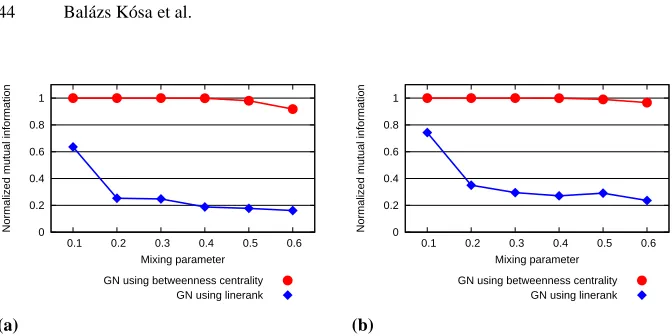
5.3. Edge Betweenness versus Edge Linerank, the Girvan-Newman Algorithm

In order to assess the applicability of the edge Linerank in practice we implemented two versions of the well-known Girvan-Newman algorithm [16] for detecting communities in a network. The first version uses edge betweenness for finding the next edge to remove from the graph as in the original paper, whereas the second applies edge Linerank for this purpose. To compare the performance of the two variants we employed normalized

mu-tual information [6], which is a frequently used measure for testing community detection

algorithms.

For two partitions_X,Y define two random variablesX andY s.t.

P(X =i) =n

X

i

n andP(Y =j) = nY_j

n ,

whereP(X =i), P(Y =j)denote the probability that a node belongs to theith_and_jth

cluster in partitions_X and_Y respectively, whilenX

i ,n

Y

j denote the number of nodes in

theseith_and_jth_{clusters, finally}_n_{is the overall number of nodes. Accordingly, the joint}

distribution of these variables is defined as

P(X =i, Y =j) = nij n ,

wherenijdenotes the number of nodes in the intersection of the aforementionedithand

jth_{clusters. The mutual information of two random variables is defined as}

I(X, Y) =H(X)−H(X|Y),

whereH(Z)denotes the Shannon entropy of random variableZ. Thus, this measure tells how much the knowledge ofY reduces the uncertainty ofX. As it is noted in [8] mutual information is not an ideal similarity measure, since for all subpartitions_Z′of partition_Z the mutual information of the derived random variablesZandZ′_{will be always the same,}

even though these subpartitions may substantially differ from each other. Therefore, in [6]

normalized mutual information is introduced

Inorm(X, Y) =

2I(X, Y) H(X)H(Y),

which equals1, if the two partitions are the same, while for independent random variables its expected value is0[8]. This observation at least partially explains the popularity of this measure for comparing community detection algorithms.

(12)

0 0.2 0.4 0.6 0.8 1

0.1 0.2 0.3 0.4 0.5 0.6

Normalized mutual information

Mixing parameter

GN using betweenness centrality GN using linerank

(a)

0 0.2 0.4 0.6 0.8 1

0.1 0.2 0.3 0.4 0.5 0.6

Normalized mutual information

Mixing parameter

GN using betweenness centrality GN using linerank

(b)

Fig. 6. (a) Effectiveness of GN algorithm versions on the benchmark graphs with larger clusters. (b) The same information for the benchmark graphs with smaller clusters.

that the correlation between the edge Linerank and betweenness values was rather low especially when the graphs contained quite definite clusters, but they did not foretell the superiority of betweenness. What is more, although these results suggest the inapplica-bility of edge Linerank for detecting clusters, since the correlation in the case of more scattered graphs was higher, the measure may still prove to be useful in certain scenarios, where the presence of clusters is not so remarkable.

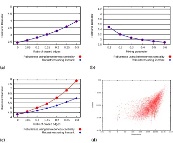
5.4. Node Betweenness versus Node Linerank, the Robustness of Networks to

Node Removal

After testing the applicability of edge Linerank we tried to find out to what degree node betweenness can be substituted with node Linerank in a practical application. For this purpose using node Linerank and betweenness we conducted the experiment of Boldi et al. again in which they tested to what extent the node removals can disrupt the structure of the web and social networks [3]. More precisely, in the course of node removalϑm edges are deleted, wheremdenotes the number of edges and0 ≤ ϑ ≤ 1. In the first step one defines an order among the nodes by using a measure and then considering the nodes in decreasing order starts to remove their incident edges. As soon as the number of the deleted edges becomes greater than or equal toϑm, the process stops. The authors were interested in how the node removal orders based on different measures influence the fraction of reachable pairs asϑincreases. They also wanted to assess the divergence between the distance distributions of the old and new graphs. They tried several different approaches to measure these changes and they have found that the relative

harmonic-diameter change reflects the differences the best. Relative harmonic-diameter is defined as

n(n−1)

P

u6=v 1

d(u,v)

,

(13)

2.5 3 3.5 4 4.5 5

0 0.05 0.1 0.15 0.2 0.25 0.3

Harmonic Diameter

Ratio of erased edges

Robustness using betweenness centrality Robustness using linerank

(a)

2.8 3 3.2 3.4 3.6 3.8 4 4.2

0.1 0.2 0.3 0.4 0.5 0.6

Harmonic Diameter

Mixing parameter

(b)

4 4.5 5 5.5 6 6.5 7 7.5 8

0 0.05 0.1 0.15 0.2 0.25 0.3

Harmonic Diameter

Ratio of erased edges

(c)

1e−06 1e−05 0.0001 0.001 0.01

0.01 0.1 1 10 100 1000 10000 100000 1e+06 1e+07

Linerank

Betweenness

(d)

(14)

contribute0 to the sum, hence this measure represents both disconnection and distance distribution [3]. For graphGdenoteR(G)its relative harmonic-diameter, then the change in this measure is calculated as

R(Q) R(P) −1,

whereP andQrespectively denotes the original graph and the graph after node removal. In our own experiments again we used both generated and real world graphs. However, in this case we increased the number of nodes of the random graphs to10000and50000. Accordingly, the sizes of the clusters also were also set higher. For the larger clusters these values ranged between40and200, whereas for the smaller clusters between20and 100. The rest of the parameters remained the same. As the diagrams in Fig. 7. (a) and (b) show the results are indistinguishable for node Linerank and betweenness. We only plotted the data belonging to the benchmarks graphs with50000nodes and larger clusters, however, the rest of the diagrams look exactly the same. Neither the changes of the mixing parameter nor the increase in the ratio of deleted edges influences this behaviour.

Nonetheless, in the case of real world graphs the scenario is somewhat less straight-forward. As one can see in Fig. 7. (c) for the CA-AstroPh dataset [15], which is the col-laboration network from the e-print ArXiv in the Astro Physics category (nodes:18772, edges: 198110), the difference between the relative harmonic-diameter change is more significant. On the other hand, as the scatter plot in Fig. 7. (d) suggests the correlation be-tween node Linerank and bebe-tweenness is still high. We experienced the same phenomenon for several real world graphs, which indicates that although the correspondence between the two measures seems to be strong, in practice one should still be careful, when node betweenness is to be substituted with node Linerank.

6. Conclusions

In our paper we compared two flow based centrality measures betweenness and Liner-ank. We have found that in the case of edges the correlation between these measures varies but tends to be rather low. Our experiments with the Girvan-Newman algorithm also underlined that edge betweenness cannot be substituted with edge Linerank in prac-tice. The results for the node variants are more promising. In our tests both Pearson’s and Spearman’s correlation coefficients were close to1in most of the cases. For the gener-ated benchmark graphs this strong correspondence persisted in the practical application in which we examined the robustness of social and web graphs to node removal. However, for real world graphs, although the correlation seemingly remained high, node between-ness outperformed node Linerank. This which shows that even in this case the substitution of the former with the latter remains problematic. Beside these investigations we have also clarified how Linerank should be computed on undirected graphs.

References

(15)

2. Adamic, L.A., Glance, N.: The political blogosphere and the 2004 u.s. election: Divided they blog. In: Proceedings of the 3rd International Workshop on Link Discovery. pp. 36–43. LinkKDD ’05, ACM (2005)

3. Boldi, P., Rosa, M., Vigna, S.: Robustness of social and web graphs to node removal. Social Netw. Analys. Mining 3(4), 829–842 (2013)

4. Brandes, U.: A faster algorithm for betweenness centrality. Journal of Mathematical Sociology 25, 163–177 (2001)

5. Brandes, U., Pich, C.: Centrality estimation in large networks. International Journal of Bifur-cation and Chaos 17(07), 2303–2318 (2007)

6. Danon, L., Duch, J., Arenas, A., D?-guilera, A.: Comparing community structure identification. Journal of Statistical Mechanics: Theory and Experiment 9008, 09008 (2005)

7. Eppstein, D., Wang, J.: Fast approximation of centrality. Journal of Graph Algorithms and Applications 8, 39–45 (2004)

8. Fortunato, S., Lancichinetti, A.: Community detection algorithms: A comparative analysis: In-vited presentation, extended abstract. In: Proceedings of the Fourth International ICST Con-ference on Performance Evaluation Methodologies and Tools. pp. 27:1–27:2. VALUETOOLS ’09, ICST (Institute for Computer Sciences, Social-Informatics and Telecommunications En-gineering) (2009)

9. Hoeffding, W.: Probability inequalities for sums of bounded random variables. Journal of the American Statistical Association 58(301), 13–30 (1963)

10. Jung, J.J.: Evolutionary Approach for Semantic-based Query Sampling in Large-scale Infor-mation Sources. InforInfor-mation Sciences. 182(1), 30–39 (2012)

11. Jung, J.J.: Measuring Trustworthiness of Information Diffusion by Risk Discovery Process in Social Networking Services. Quality & Quantity. 48(3), 1325–1336 (2014)

12. Kang, U., Papadimitriou, S., Sun, J., Tong, H.: Centralities in large networks: Algorithms and observations. In: SDM. pp. 119–130. SIAM / Omnipress (2011)

13. Keszler, A., Szir´anyi, T.: A mixed graph model for community detection. Int. J. Intell. Inf. Database Syst. 6(5), 479–494 (Sep 2012)

14. Lancichinetti, A., Fortunato, S., Radicchi, F.: Benchmark graphs for testing community detec-tion algorithms. Phys. Rev. E 78(4) (2008)

15. Leskovec, J., Kleinberg, J., Faloutsos, C.: Graph evolution: Densification and shrinking diam-eters. ACM Trans. Knowl. Discov. Data 1(1) (2007)

16. Newman, M.E.J., Girvan, M.: Finding and evaluating community structure in networks. Phys. Rev. E 69(2) (2004)

17. Page, L., Brin, S., Motwani, R., Winograd, T.: The pagerank citation ranking: Bringing order to the web. In: Proceedings of the 7th International World Wide Web Conference. pp. 161–172 (1998)

18. Pham, X.H., Jung, J.J.: Recommendation System Based on Multilingual Entity Matching on Linked Open Data. Journal of Intelligent & Fuzzy Systems 27(2), 589–599 (2014)

19. Vossen, G.: Big data as the new enabler in business and other intelligence. Vietnam Journal of Computer Science 1(1), 3–14 (2014)

20. Yakoubi, Z., Kanawati, R.: Licod: A leader-driven algorithm for community detection in com-plex networks. Vietnam Journal of Computer Science 1(4), 241–256 (2014)

(16)

practice, tree and graph transformers, semantic web, big data, network analysis and data mining.

Márton Balassi was born in 1990. In 2014 he graduated (MSc) with distinction from the Department of Information Systems of the Faculty of Informatics at Eötv ös Loránd University. Currently he is pursuing a PhD at a group focused on data intensive and dis-tributed algorithms at the Informatics Laboratory of the Hungarian Academy of Sciences, Institue for Computer Science and Control. In addition he is an active committer and project management committee member of Apache Flink, an open-source framework for efficient distributed data processing.

Péter Englert was born in 1990. Currently he is a Master’s student at the Department of Information Systems of the Faculty of Informatics at Eötv ös Loránd University. He has been involved in research from a wide range of areas, including ecological simulations, mathematical modeling and chemoinformatics. His current work focuses on distributed algorithms and graph databases.

Attila Kiss was born in 1960. In 1985 he graduated (MSc) as mathematician at Eötv ös Loránd University, in Budapest. He defended his PhD in the field of database theory in 1991; his thesis title was Dependencies of Relational Databases. Since 2010 he is working as the head of Information Systems Department at Eötv ös Loránd University. His scien-tific research is focusing on database theory and practice, semantic web, big data, graph databases, data mining. In addition, he also investigates questions related with social net-work analysis.