Efficient Processing of Continuous Queries Utilizing
F-relationship in Stock Databases
Sanghyun Park1, You-min Ha2, Chihyun Park3 and Sang-Wook Kim4
1Faculty of Computer Sciences, Yonsei University [email protected]
2Software Center of Samsung Electronics Co., Ltd. [email protected]
3Korea Institute of Science and Technology Information [email protected]
4Faculty of Computer Science and Engineering, Hanyang University [email protected]
Abstract. This paper analyzes the properties of user queries in a system for stock investment recommendation, and defines the F-relationship, which is a new type of a relationship between two queries. A query is composed of user defined conditions for an interesting stock item and is systematically invoked whenever the price of that stock item is changed. An F-relationship between two queries Q1 and Q2 means that, if the recommendation type of a preceding query Q1 is X, then its following query Q2 always has X as its recommendation type, where the recommendation type is one of SELL, HOLD, BUY, and NONE. If there is an F-relationship between Q1 and Q2, the recommendation type of Q2 is decided immediately by that of Q1, therefore we can keep Q2 from being actually processed. To exploit this fact, we suggest two methods in this paper. The former analyzes all the F-relationships among user queries in the system and represents them as a graph. The latter searches the graph and decides the order of queries to be processed, which makes the number of unexecuted queries maximized. With these methods, a large portion of user queries are not actually processed. As a result, the performance of processing all the queries is greatly improved. We examined the superiority of the suggested methods through a variety of experiments using real-world stock market data. According to the results of our experiments, the overall time of continuous query processing with our proposed methods has reduced to less than 10% of that with the traditional method.
Keywords: Stock databases, Continuous query processing, F-relationship
1.
Introduction
Stock price sequences are a typical example of time-series data [1], [5], [7], [9], [20]. Since the goal of stock investors is to earn high return, it would help investors achieve successful stock investments to recommend proper buying and selling points via analysis of the stock price sequences [10], [17], [21]. However, it is not easy for investors to determine appropriate buying and selling points themselves for earning high return in such environment where stock prices fluctuate significantly everyday [13].
Each stock investor has his/her own conditions for buying or selling stocks. Some investors want to earn high return in spite of high risk while others do not accept high risk for high return. To meet requirements of a variety of stock investors, it would be so useful to develop a system that automatically recommends stock items whose price changing patterns come to satisfy the conditions required by individual investors.
There have been several attempts to efficiently identify frequent patterns of price changing from stock data. Traditional pattern matching from a time-series stream dataset such as stock history is highly time-consuming and is not suitable for recognizing irregular patterns. To overcome these weak points, [24] proposed an efficient pattern matching approach. This approach extracts partial time points as features which can help to determine the similarity of patterns based on the notion of perceptually important point (PIP). Then, with these reduced features, Spearman‟s rank correlation coefficient is used to measure the similarity between the input segment and the previously detected patterns. This approach aims to improve the efficiency of pattern matching itself. However, this approach is not specifically applicable to real-world stock databases because it cannot consider several variables including recommendation types required in stock trading systems. Another study related to our approach focused on detecting frequent patterns and predicting the trend corresponding to an input pattern in a financial time-series dataset such as stock history [25]. This study could be applied in recommending both buying and selling actions. However, this study primarily focused on improving the accuracy of predictions without building the practical recommendation systems for investment.
In our previous work [12], we developed a system that recommends investment types to stock investors by discovering useful rules from past changing patterns of stock prices in a database. In this system, we defined a new model which could recommend stock investment types according to the frequent pattern of pricing of a stock item. This allows investors to impose various conditions on rule bodies flexibly, and also improves the performance of a rule discovery process by reducing the number of rules to be discovered. For efficient discovery and matching of rules, we proposed methods for discovering frequent patterns, constructing a frequent pattern base, and indexing those patterns. We also suggested a method that efficiently finds the rules matched to a query from a frequent pattern base, and proposed a method that recommends an investment type by using the rules.
In this paper, we discuss efficient processing of a large number of continuous queries for stock investment recommendation. First, we search for the Follows-relationship (F-relationship in short), which is a new type of a (F-relationship between two queries, by analyzing properties of user queries. An F-relationship between two queries Q1 and Q2 under a recommendation type X implies that, if a preceding query Q1 has X as a recommendation type, then its following query Q2 always has X as its recommendation type. When there exists an F-relationship between Q1 and Q2, the recommendation type of Q2 is decided immediately by that of Q1, therefore we can safely keep Q2 from being processed. For achieving this, we propose a method that finds all the F-relationships among user queries and represents them as a graph. We also propose a method that searches the graph and decides the order of queries to be processed, which makes the number of unexecuted queries as many as possible. With our methods, a large portion of user queries get free from actual processing. As a result, the performance of processing all the queries is greatly improved. According to our experimental results, more than 90% of queries are waived from actual processing with our methods.
The organization of the paper is as follows. Section 2 briefly reviews the rule model proposed in our previous work. Section 3 discusses the performance problems occurring in our target application environment. Section 4 presents the methods for solving the problems. Section 5 verifies the effectiveness of our proposed methods via extensive experiments. Finally, Section 6 summarizes and concludes the paper.
2.
Stock Investment Recommendation System
In this section, we explain the rule model and the query model proposed in reference [12].
2.1. Rule model
In this paper, we use the following form of a rule to express the trend of changing stock prices. Here, H and B denote a rule head and a rule body, respectively. This rule implies that B happens after time t since H has occurred.
Next, we discuss (s, c) in the rule. A changing pattern can be formed as a rule head only when a sufficient number of stock sequences support the pattern. s defined in the following is called a support, which means how many times the pattern P corresponding to H appears in past stock sequences [2], [3].
100 match that patterns of that as same is length whose patterns of s occurrence # match that patterns of s occurrence # = ) ( H H H s
Also, for being formed as a rule, a set of sequences that satisfy the above support should show a similar tendency in the time range of the rule body. c defined below is called a confidence, which represents how many stock sequences matched to H satisfy the condition on B together [2].
Our approach discovers those rules whose support and confidence are both larger than predetermined thresholds during analyzing the past stock sequences. If a recent changing pattern of an investor's stock item of interest is matched to some H, it recommends an investment type by referring to its B. Possible investment types to be recommended are „BUY‟, „SELL‟, „HOLD‟, and „NO RECOMMENDATION‟. They are decided by conditions for B, which are highly dependent on propensities of investors.
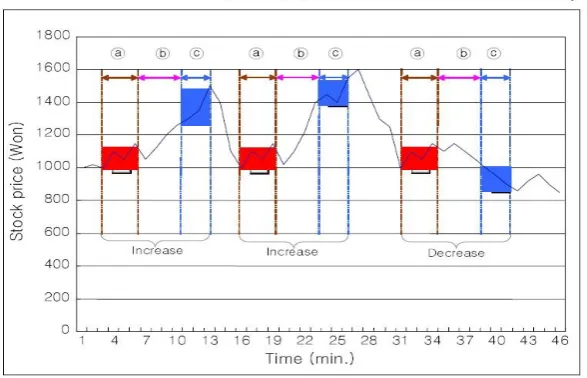
Fig. 1. An example showing the rule model.
Figure 1 shows a simple example of a stock price change. In this stock data, a pattern in the time interval ⓐ occurs three times. After a time interval ⓑ since then, the price is shown to increase twice and is shown to decrease once. From this fact, if a pattern in the time interval ⓐ appears again, the system recommends „BUY‟ as an investment type for this stock because the price is likely to increase with probability of 0.66. In this example, we regarded a pattern occurring three times as frequent. However, the system regards a pattern frequent only when its support is more than a minimum threshold, thereby considering it to be a rule head [2], [3].
In stock applications, H is an event corresponding to an appearance of a pattern P within the time range of the rule head as shown in the time interval ⓐ of Figure 1. Also, B is an event that corresponds to the characteristics of stock prices within the time range
100 match
that patterns of s occurrence #
of conditions e
satisfy th and
match that patterns of s occurrence #
= ) ,
(
H
B H
of the rule body as shown in Figure 1. In Figure 1, for example, B can be represented as „INCREASE‟.
Like this, stock investors specify their own conditions, which are related to the investment types for recommendations, on the characteristics of stock prices within the time range of the rule body. Such conditions are called rule body conditions, which decide when the characteristics of stock prices are regarded as „INCREASE‟. In the prior example, investors set the rule body condition as “the average stock price in the time range of the rule body increases more than 20% in comparison with the last stock price in the time range of the rule head”. In this case, the changing patterns of stock prices in Figure 1 are discovered as a meaningful rule. We note that these rule body conditions vary depending on dispositions of investors.
The value ranges of elements may differ from one stock sequence to another. In addition, even within a single stock sequence, the element values may fluctuate a lot in response to economic situations or changes in business revenue. Therefore, it is rarely possible for a stock sequence with raw element values to contain frequent patterns. To solve this problem, we take the approach to transform a raw stock sequence into a sequence of change ratios and then into a symbol sequence. Also, we build an index on the frequent patterns discovered for efficient processing of continuous queries at every update period of stock prices.
Before continuous query processing starts, investors define all their conditions for B. They are stock items of interest, acceptable price changing rates for buying and selling conditions, and so on. As mentioned earlier, however, these conditions vary according to investors. For example, an investor wants the system to recommend „BUY‟ when the average price in the time range of the rule body gets more than 20% high against the last price in the time range of the rule head. On the other hand, another investor wants the system to recommend „BUY‟ when the lowest price in the time range of the rule body gets more than 10% high against the last price in the time range of the rule head. Moreover, we note that, even for the same investor, such conditions are changeable according to her/his investing points.
2.2. Query model
A query Q for requiring recommendation types and its result FQ are formally defined as follows.
Definition 1. Q, query form
A query Q for requiring recommendation types is formulated in the following form.
Each variable has the meaning as below.
• I : the stock item of interest.
• T : the time interval between the end of a rule head and the beginning of a rule body.
)
],
,
[
,
,
,
(
=
I
T
BL
mC
• BL : the length of a rule body.
• [α, β]: the range of average increase ratio for retaining the current stock item. Their actual meanings will be explained in Definition 2.
• mC : the minimum confidence, which is set to more than 0.5. The reason for this setting will be also explained in Definition 2.
The system executes a query Q whenever the price of a stock item I is changed. If the pattern obtained so far is matched to some frequent pattern, it recommends an appropriate investment type by referring to the corresponding rule bodies. This is a kind of continuous query processing because it processes the same query continuously according to data updates. The result of each query processing, F(Q) , has the following value.
Definition 2. F(Q), the result of processing a query Q
For every case that supports the rule head, which is matched to Q, we calculate its average increase ratio r by comparing the end price of the rule head to the average price of the rule body. As a result, F(Q) for query Q=(I, T, BL, [α, β], mC), is defined as follows.
where α and β are the minimum and maximum values for selecting „HOLD‟, respectively. The recommendation type, X, is determined as follows.
•SELL: If the ratio of cases satisfying (r≤ α) is larger than mC.
•HOLD: If the ratio of cases satisfying (α ≤ r≤ β) is larger than mC.
•BUY: If the ratio of cases satisfying (r ≥ β) is larger than mC.
•NONE: Otherwise (All three ratios are less than mC)
As stated in Definition 1, mC is required to set to at least 0.5 in order to avoid more than one investment type from being recommended. When F(Q) has a value of X, we denote it as F(Q)=X and read it as “X is recommended as a result of processing query Q.”
The proposed approach enables stock investors to easily adapt the query model to suit their needs or application environments. Thus, it provides a fundamental framework for adaptive recommendation systems for stock investment. According to the experimental results, the system provides more than 70% satisfaction ratio in most cases, and its response times are much less than a second, which is tolerable even in on-line environment [12].
3.
Motivation
In this section, we characterize our target application environment, and point out the performance problems occurring in this environment. Then, we present an example that explains a core idea for solving those problems.
First, as a target data for discovering rule heads, we use real-world stock price data },
, , , { , = )
(Q X X SELL HOLDBUY NONE
collected for 20 years. From the data, we store frequent patterns, which are used as rule heads, in a database, and build an index on these rule heads for efficient query processing. The price of each stock item is periodically updated in a database. At every update time, the most recent prices of each stock item are used in a query to inquire whether they are matched to some frequent patterns. If a matched frequent pattern is found in the database of rule heads, an appropriate investment type for the stock item is computed and recommended. The conditions for determining a rule body are different according to queries. Thus, in order to compute the average increase ratio, we need to access all the sequences that support the rule head. This causes a large number of random accesses from disk.
Also, there are a lot of stock investors in our target application environment. Each investor might have multiple stock items of interest, thereby issuing multiple queries in the system. All the queries requested by investors are stored and executed in main memory, and are periodically stored into the disk for the purpose of backup. As a result, there are a great number of queries to be processed continuously in every update period. This is a very important issue of continuous query processing dealt with in stream data management [6], [19].
Let us consider two queries Q1 = („Samsung Electronics‟, 0, 1, [-0.01, 0.01], 0.7) and
Q2 = („Samsung Electronics‟, 0, 1, [-0.02, 0.02], 0.6) where the stock item, the time interval, and the length of a rule body are identical. If F(Q1) is „HOLD‟, this implies that, for all the cases matched to a rule head, more than 70% cases have their price increase rate between -0.01 and 0.01. Because queries Q1 and Q2 have the stock item, the time interval, and the length of a rule body in common, the rule head and body to be examined in query processing is also identical in the two queries. So, since it recommends „HOLD‟ when the ratio of cases whose price increase rate is between -0.01 and 0.01 is more than 70%, we can safely regard that F(Q2) is also „HOLD‟ without processing Q2.
There are a large number of user queries, each of which should be processed once within every update period of stock prices. As a clue to this problem situation, we have to pay attention to the relationship between Q1 and Q2.
4.
Query Processing with F-Relationship
This section discusses the F-relationship among queries, and proposes a method that reduces the number of queries to be actually processed by using the relationship.
4.1. F-relationship
In this section, we define the relationship, and suggest some conditions for the F-relationship held.
Definition 3: F-relationship and a set of F-relationships
defined as follows.
We read R(Q1, Q2, X) as „Q2 follows Q1 for recommendation type X‟, where Q1 is a
preceding query, and Q2 is its following query. Also, a set of F-relationships related to a preceding query Q1 and a recommendation type X is denoted as FRS(Q1, X).
If the recommendation type of a preceding query Q1 is X, then the following query Q2 always has X as its recommendation type. If there exists an F-relationship between Q1 and Q2, the recommendation type of Q2 is decided immediately by that of Q1, therefore we can keep Q2 from being actually processed. We suggest two methods in this paper. The former analyzes all the F-relationships among user queries and represents them as a graph. The latter searches the graph and decides the order of queries to be processed, which makes the number of unprocessed queries maximized. With these methods, most of user queries are kept from actual processing.
Given a query Q=(I, T, BL, [α, β], mC), the system processes Q and provides a recommendation type whenever a new price of stock item I arrives. When different users issue queries on the same stock item I, there could exist a number of F-relationships among those queries.
Theorem 1: F-relationship, R(Q1, Q2, X)
Two queries having the same stock item I, time interval T, and rule body length BL can be expressed as follows.
In this case, there can be three possible F-relationships between these two queries.
1. IF (α1≤ α2) AND (mC1 ≥ mC2) AND F(Q1)=SELL, THEN F-relationship R(Q1, Q2,
SELL) always holds.
2. IF (α1 ≥ α2) AND (β 1 ≤ β 2) AND (mC1 ≥ mC2) AND F(Q1)=HOLD, THEN F-relationship R(Q1, Q2, HOLD) always holds.
3. IF (β 1≥ β 2) AND (mC1 ≥ mC2) AND F(Q1)=BUY, THEN F-relationship R(Q1, Q2,
BUY) always holds.
Proof: For proving Theorem 1, let us depict [α1, β1] and [α2, β2] of Q1 and Q2. Without loss of generality, we assume α1≤ α2 here.
We calculate the average increase rate by comparing the end price of the rule head to the average price of the rule body. If it is less than α1, this case supports F(Q1)=SELL. If
. = ) ( then , = ) ( If ) , ,
(Q1 Q2 X F Q1 X F Q2 X
R ) ], , [ , , , (
= 1 1 1
1 I T BL mC
Q
) ], , [ , , , (
= 2 2 2
2 I T BL mC
the number of occurrences matched to the rule head is n, the confidence, C1(SELL), for the number of cases recommending F(Q1)=SELL, r1(SELL), is computed as below.
If C1(SELL) ≥ mC1, then F(Q1)=SELL always holds. For Q1, we assume F(Q1)=SELL. According to the definition, the number of cases belonging to S1, r1(SELL), is expressed as follows.
As in the figure above, since S1 ⊆ S2, the number of cases belonging to S2, r2(SELL), is always larger than or equal to r1(SELL).
Therefore, we obtain the following inequality.
As in the definition C1, since C2(SELL)=r1(SELL)÷n, we obtain the following equation.
Because C2(SELL) ≥ mC2, we easily know that F(Q2)=SELL. As a result, if (α1≤ α2) AND (mC1 ≥ mC2) AND (F(Q1)=SELL), F-relationship R(Q1, Q2, SELL) does always hold. We can also prove Theorems 1.2 and 1.3 in the similar fashion.
In our system, a large number of queries might have F-relationships with one another. As stated earlier, the recommendation type of a following query is automatically determined by that of its preceding query. Therefore, we can safely omit the expensive processing of those following queries.
4.2. Composition of a query set
F-relationships among queries can be expressed by using directed graphs where vertices represent queries and directed edges represent F-relationships of a recommendation type. For example, F-relationship R(Q1, Q2, BUY) is expressed by a directed graph shown in Figure 2.
When there are n queries, the maximum number of outgoing edges from a given query is n-1. Therefore, the space complexity for storing the direct edges to express all the possible F-relationships of n queries is O(n2). As a result, the storage cost becomes high when n is large, and thus needs to be reduced.
n
SELL
r
SELL
C
1(
)
=
1(
)
1 1
1
(
SELL
)
=
n
C
(
SELL
)
n
mC
r
)
(
)
(
12
SELL
r
SELL
r
2 1
1
2
(
SELL
)
r
(
SELL
)
n
mC
n
mC
r
2 2
2
2
(
SELL
)
=
r
(
SELL
)
n
n
mC
n
=
mC
Fig. 2. A directed graph for F-relationship R(Q1, Q2, BUY)
Let us consider a direct graph shown in Figure 3(a). This graph expresses three F-relationships R(Q1, Q2, BUY), R(Q2, Q3, BUY), and R(Q1, Q3, BUY). Since the third F-relationship (i.e., R(Q1, Q3, BUY)) is derivable from the first two F-relationships, it can be deleted from the directed graph without any information loss. We call such an F-relationship derivable F-relationship. The graph obtained after removing all the derivable F-relationships from the graph in Figure 3(a) is shown in Figure 3(b).
Fig. 3. A direct graph and its concise representation
The set of F-relationships obtained after removing all the derivable F-relationships from FRS(Q, X), a set of F-relationships having Q as their preceding query and X as their recommendation type, is formally defined as follows:
Definition 4: Set of core F-relationships, coreFRS(Q, X)
Given a query Q and a recommendation type X, let FQS(Q, X) denote a set of all the queries Qi(≠Q) which satisfy the F-relationship R(Q, Qi, X) and let nonCoreFQS(Q, X) denote a set of all the queriesQi (≠Q) which satisfy the F-relationship R(Qr, Qi, BUY) for some Qr in FQS(Q, X). Then, the set of core F-relationships coreFRS(Q, X) is defined as
As shown in Figure 3, when there exists an F-relationship R(Q1, Q2, X), the
containment relationship FRS(Q1, X) ⊃ FRS(Q2, X) is always satisfied. As described in ( , )
( ,
) =
( ,
)
Qi nonCoreFQS Q X( ,
i,
)
Algorithm 1, the set of core F-relationships coreFRS(Q, X) is easily obtained by using this property.
Algorithm 1: get_coreFRS(Q, X) for obtaining the set of core F-relationships coreFRS(Q, X)
Input : Query Q, Recommendation type X
Output : Set of core F-relationships coreFRS(Q, X) 1 coreFRS(Q, X) := FRS(Q, X);
2 foreachQi ∈ nonCoreFQS(Q, X) do
3 coreFRS(Q, X) := coreFRS(Q, X) - {R(Q, Qi, X)}; 4 return coreFRS(Q, X)
If an investor submits a new query Q, we first obtain FRS(Q, X), for each recommendation type X and then take only coreFRS(Q, X) by using the algorithm get_coreFRS(Q, X) shown above. Then, for each element R(Q, Qi, X) in coreFRS(Q, X), we retrieve all the queries Qr satisfying R(Qr, Qi, X) and replace R(Qr, Qi, X) with R(Qr, Q, X) in the existing set of F-relationships.
Let us consider the time complexity of inserting a new query Q into a system with n queries. The maximum number of F-relationships R(Q, Qi, X) in coreFRS(Q, X) is n, and the maximum number of queries Qr satisfying R(Qr, Qi, X) is n-1 when Qr is excluded. Therefore, the total time can be expressed asymptotically as O(n(n-1)) = O(n2). However, when inserting a new query Q into an existing system, we only consider the queries whose target stock item, time interval, and length of rule body are same as those of Q and thus the actual time cost is expected to be not much.
Now, let us consider the space complexity of the data structure for expressing relationships. With the assumption that every query maintains just the set of core F-relationships, let us examine the maximum number of F-relationships an arbitrary query Q can have. When F(Q)=SELL, there can be two types of following queries at most; (1) following queries that have the same mC value but a larger α value, and (2) following queries that have the same α value but a smaller mC value. When F(Q)=BUY, there can be also two types of following queries at most. When F(Q)=HOLD, following queries may have two identical values and one different value among mC, α, and β. That is, the maximum number of types of following queries is 3. Therefore, the maximum number of the following queries having Q as their preceding query is 7, and thus the space complexity at the worst case becomes O(7n) = O(n).
4.3. Determination of a query processing order
required for performance improvement to determine their execution order that can minimize the total query processing cost.
If we select a query Q with the largest set of F-relationships FRS(Q, X) and execute it first, then there can be a large number of queries processed indirectly. However, unless F(Q) = X, indirect processing is infeasible even though there are lots of queries included in FRS(Q, X). In addition, the approach to maintain FRS(Q, X) for every pair of a query Q and a recommendation type X requires high storage cost. Because of these two reasons, we do not take the approach to process the queries in the order of the size of their F-relationship sets.
An alternative criterion to the size of F-relationship sets for determining the execution order of queries is the minimum confidence of queries. When two queries are given, the parameters to decide whether or not they are in F-relationships are their change ratio of retention [α, β] and their minimum confidence mC. Among these three parameters, the minimum confidence is the only one that can determine the order of F-relationships irrespective of a recommendation type. That is, a query with a higher minimum confidence can be a preceding query of another query with a lower minimum confidence regardless of a recommendation type, but the reverse situation is not possible. Therefore, we can highly expect that the queries with a higher minimum confidence have a larger set of F-relationships. Based on this reasoning, we decide to execute the queries with a higher minimum confidence prior to the queries with a lower minimum confidence so as to increase the chance of indirect query processing via the F-relationship. Algorithm 2 shown below determines the execution order of queries according to their minimum confidence and then processes them in the execution order.
When a user submits a new query into a set QS of queries whose I, T, and BL values are identical to those of the new query, the cost to insert the new query to the sorted list of QS is O(logn); therefore it does not significantly affect the construction cost (i.e., O(n2)) of a query set mentioned in Section 4.2.
Algorithm 2: selectQuery(QS) for determining the execution order of queries according to their minimum confidence and then processing them according to their execution order
Input : set QS of queries with identical I, T, and BL values
Output : none
1 While QSis not emptydo
2 Q := query with the highest minimum confidence among the elements of QS; 3 delete Q from QS;
4 ifthe valueofF(Q) is not decided yetthen
5 process F(Q) directly; 6 X := F(Q);
5.
Performance Evaluation
In this section, we verify the superiority of the proposed approach via experimental performance evaluation.
5.1. Experimental environment
We evaluated the performance of the proposed approach using real-world stock price data. To collect actual stock price data, we recorded the prices of 905 KOSPI [16] stock items every minute for about three months. For each individual stock item, we created a query set by combining the following parameters.
• α: chosen among -0.003, -0.002, and -0.001 • β: chosen among 0.001, 0.002, and 0.003 • T: fixed at 0
• BL: chosen among 1, 3, and 5
• mC: chosen among 50%, 60%, 70%, and 80%
By combining the above parameters, we created 108(=3ⅹ3ⅹ3ⅹ4) queries for each stock item and 97,740(=108ⅹ905) queries in total. All experiments were performed on the PC equipped with Intel Pentium 2.4GHz CPU, 1GB memory, 80GB HDD, and Window 2003 Server operating system.
To evaluate the hit ratio of the proposed model, we had measured satisfaction ratio and recommendation ratio with various independent variables in the reference [12]. In this study, however, we designed and performed experiments to evaluate how much the query processing performance is improved by the application of F-relationships among queries. Therefore, we excluded the experiments on the parameters (i.e., T and BL) which are not related with the query processing performance.
5.2. Experimental result
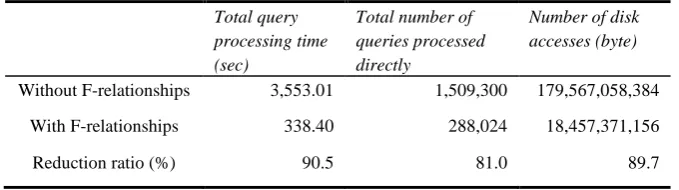
Performance improvement by utilizing F-relationships. For the two cases of processing all queries with and without the utilization of F-relationships, Table 1 shows the time for processing all queries, the number of queries processed directly, and the number of disk accesses.
Table 1. Time for processing all queries, number of queries processed directly, and number of disk accesses with or without the utilization of F-relationships
Total query processing time (sec)
Total number of queries processed directly
Number of disk accesses (byte)
Without F-relationships 3,553.01 1,509,300 179,567,058,384
With F-relationships 338.40 288,024 18,457,371,156
Reduction ratio (%) 90.5 81.0 89.7
The time for processing all queries with the application of F-relationships is reduced to 9.5% of that without the application of F-relationships. This verifies the significant improvement in query processing performance. Let us now consider the number of queries processed directly. About 1.22 million queries among about 1.5 million queries were not processed directly; instead, their recommendation types were determined indirectly by the application of F-relationships.
However, extra time is required for utilizing F-relationships. Therefore, we may expect that the reduction ratio of the time for processing all queries is less than 81%, which is the reduction ratio of queries processed directly to the total queries. However, in this experiment, we observed that the reduction ratio of the time for processing all queries is about 90%. We can think of the two reasons for this higher reduction ratio; the first reason is that the time for processing each individual query may not be identical, and the second reason is that the time for disk accessing dominates the time for query processing. In Table 1, we can observe that the reduction ratio of the time for processing all queries is almost same as the reduction ratio of the size of disk accesses, and this observation supports our conjecture.
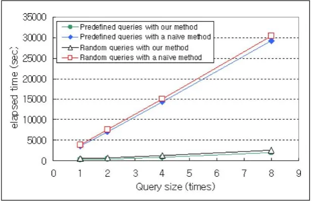
Fig. 4. Processing time with increasing number of queries
Figure 4 shows that the time for processing random queries with our approach is larger than that for processing predefined queries with our approach. This is because more predefined queries than random queries are processed indirectly in our approach. However, with our approach, the difference between the time for processing all predefined queries and the time for processing all random queries is not that large. This result verifies that the set of predefined queries used throughout the experiments has not been manipulated to show off the performance improvement of our approach.
Let us examine Figure 4 again. When F-relationships among queries are not applied, every query must be processed directly, and thus it takes long time to process all the predefined or random queries. Note that the processing time without the usage of F-relationships for all predefined queries is not much different from that for all random queries. This is because the number of predefined queries processed directly is almost same as that of random queries. On the other hand, it is clearly shown in Figure 4 that the time for processing queries with the usage of F-relationships is much smaller than that without the usage of F-relationships, and the difference becomes larger as the number of queries increases. This experiment revealed that our approach improves the query processing performance up to 14 times compared to the existing one.
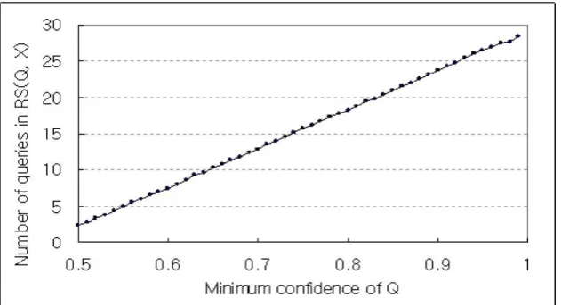
We observed that the average number of queries in F-relationships FRS(Q, X) increases linearly in proportion to the minimum confidence of query Q. Actually, the correlation coefficient of these two variables was 0.99, and thus we found out that the two variables have extremely positive correlation. Therefore, we can deduce that the processing order of queries determined by their minimum confidences should be almost same as that determined by the size of the F-relationship set.
Fig. 5. Average number of queries in F-relationships with the increasing minimum confidence
6.
Conclusion
In this paper, we have discussed continuous query processing for stock investment applications. The approaches proposed in previous studies construct the rules from stock databases, predict the price change patterns of the stocks in which investors are interested, and then recommend one of three investment types (i.e., HOLD, BUY, and SELL) to the investors. For doing these, the previous approaches define new rule models, and then construct the rules when the trends matched to frequent price change patterns satisfy the investment conditions of investors. Here, frequent patterns are used as rule heads and their succeeding price change patterns are used as rule bodies.
and the other for determining the query processing order by which the F-relationships constructed in the previous step can be applied effectively.
To demonstrate the superiority of our approaches, we compared the approach with and without the usage of F-relationships by extensive experiments using real-world stock data. The result revealed that the time for processing all queries with the usage of F-relationships was just 10% of that without the usage of F-F-relationships.
As a further study, we are planning to extend our approach to the environment where a stock database is updated dynamically [21] and its frequent pattern base should be updated accordingly.
Acknowledgement. This work was supported by the National Research Foundation of Korea (NRF) grant funded by the Korea government (MSIP) (NRF-2014R1A2A1A10054151) and the Ministry of Science, ICT and Future Planning (MSIP), Korea, under the Information Technology Research Center (ITRC) support program (IITP-2015-H8501-15-1013) supervised by the Institute for Information & communication Technology Promotion (IITP).
References
1. Agrawal, R., Lin, K.-I., Sawhney, H. S., Shim, K.: Fast Similarity Search in the Presence of Noise, Scaling, and Translation in Time-Series Databases. In proceedings of the 20th International Conference on Very Large Databases. Zurich, Switzerland, 490-501. (1995) 2. Agrawal, R., Srikant, R.: Mining Sequential Patterns. In proceedings of the 11th
International Conference on Data Engineering, Taipei, Taiwan, 3-14. (1995)
3. Agrawal, R., Srikant, R.: Fast Algorithms for Mining Association Rules. In proceedings of the 20th International Conference on Very Large Databases. Morgan Kaufmann, Santiago, Chile, 487-499. (1994)
4. Agrawal, R., Faloutsos, C., Swami, A.: Efficient Similarity Search in Sequence Databases. In proceedings of the 4th International Conference on Foundations of Data Organization and Algorithms. Chicago, Illinois, USA, 69-84. (1993)
5. Anderson, T. : The Statistical Analysis of Time Series. Wiley (1971)
6. Babu, S., Widom, J.: Continuous Queries over Data Streams. ACM SIGMOD Record, Vol. 30, No. 3, 109-120. (2001)
7. Baheti, A., Toshniwal, D.: Trend Analysis of Time Series Data Using Data Mining Techniques, In proceedings of the 3rd International Congress on Big Data. Anchorage, Alaska, USA, 430-437, (2014)
8. Bloomfield, P.: Fourier Analysis of Time Series. Wiley (2000)
9. Faloutsos, C., Ranganathan, M., Manolopoulos, Y.: Fast Subsequence Matching in Time-Series Databases. In proceedings of the 21th ACM International Conference on Management of Data. Minneapolis, Minnesota, USA, 419-429, (1994)
10. Fu, T., Cheung, T., Chung, F., Ng, C.: An Innovative Use of Historical Data for Neural Network Based Stock Prediction. In proceedings of the 6th International Conference on Information Sciences. Reading, UK, (2006)
11. Garg, B., Beg, M. M. S., Ansari, A. Q.: Fuzzy Time Series Model to Forecast Rice Production. In the proceedings of the 22th International Conference on Fuzzy Systems. Hyderabad, India, 1-8. (2013)
12. Ha, Y. M., Kim, S. W., Park, S.: Rule Discovery and Matching in Stock Databases. Information and Software Technology, Vol. 51, Issue 7, 1140-1149. (2009).
14. Kim, S. W., Park, S., Chu, W. W.: An Index-Based Approach for Similarity Search Supporting Time Warping in Large Sequence Databases. In the proceedings of the 17th International Conference on Data Engineering . Heidelberg, Germany, 607-614. (2001) 15. Kim, S. W., Shin, M.: Subsequence Matching Under Time Warping in Time-Series
Databases: Observation, Optimization, and Performance Results. International Journal of Computer Systems Science & Engineering, Vol. 23, No. 1. (2008)
16. Koscom Data Mall, http://datamall.koscom.co.kr (2005)
17. Kwon, Y., Choi, S., Moon, B.: Stock Prediction Based on Financial Correlation. In proceedings of the 7th annual conference on Genetic and Evolutionary Computation. Washington, DC, USA, 2061-2066. (2005)
18. Loh, W. K., Kim, S. W., Whang, K. Y.: A Subsequence Matching Algorithm that Supports Normalization Transform in Time-Series Databases. Data Mining and Knowledge Discovery Journal, Vol. 9, No. 1, 5-28. (2004)
19. Manku, G., Motwani, R.: Approximate Frequency Counts over Data Streams. In proceedings of the 28th International Conference on Very Large Data Bases. Hong Kong, China, 346-357. (2002)
20. Moon, Y. S., Loh, W. K.: Efficient Stream Subsequence Matching Algorithms for Handheld Devices on Streaming Time-Series Data. International Journal of Computer Systems Science & Engineering, Vol. 24, No. 4. (2009)
21. Sehgal, V., Song, C.: SOPS: Stock Prediction Using Web Sentiment. In proceedings of the International Conference on Data Mining Workshop, Omaha, Nebraska, USA, 21-26. (2007) 22. Suematsu, N., Hayashi, A.: Time Series Alignment with Gaussian Processes. In proceedings
of the 21th International Conference on Pattern Recognition, Tsukuba, Japan, 2355-2358. (2012)
23. Park, S., Chu, W. W., Yoon, J., Hsu, C.: Efficient Searches for Similar Subsequences of Difference Lengths in Sequence Databases. In proceedings of the 16th IEEE International Conference on Data Engineering, San Diego, California, USA, 23-32. (2000)
24. Xie, Y., Wulamu, A., He, Q., Liu, X.: Time Series Prediction Method Based on Pat-tern Matching. Journal of Computational Information Systems, Vol.10, No.13, 5773-5784. (2014)
25. Wu, K.P., Wu, Y.P., Lee, H.M.: Stock Trend Prediction by Using K-Means and AprioriAll Algorithm for Sequential Chart Pattern Mining. Journal of Information Science and Engineering, Vol.30, 653-667. (2014)
Sanghyun Park is now a Professor in Department of Computer Science, Yonsei University, Seoul, Korea. He received the BS and MS degrees in computer engineering from Seoul National University in 1989 and 1991, respectively. He received PhD degree in the Department of Computer Science from University of California at Los Angeles (UCLA) in 2001. His current research interests include database, data mining, bioinformatics, and flash memory.
You-min Ha is now a Senior Software Engineer in Software Center of Samsung Electronics Co., Ltd., Korea. He received the BS and MS degrees in computer science from Yonsei University, Seoul, Korea in 2004 and 2007 respectively. His interest includes data mining, database system and human-behavior pattern recognition.
from Yonsei University, Seoul, Korea in 2013. His current research interests include bioinformatics, data mining, and database system.
Sang-Wook Kim (corresponding author) received the B.S. degree in Computer Engineering from Seoul National University at 1989, and earned the M.S. and Ph.D. degrees in Computer Science from KAIST at 1991 and 1994, respectively. From 1995 to 2003, he served as an Associate Professor at Kangwon National University. In 2003, he joined Hanyang University, Seoul, Korea, where he currently is a Professor in Department of Computer Science and Engineering and the director of the Brain-Korea-21-Plus research program. His research interests include databases, data mining, multimedia information retrieval, social network analysis, recommendation, and web data analysis.