A Novel Self-adaptive Grid-partitioning Noise
Optimization Algorithm Based on Differential Privacy
Zhaobin Liu1, Haoze Lv1, Minghui Li1, Zhiyang Li1, and Zhiyi Huang2 1 School of Information Science and Technology, Dalian Maritime University
China
Correspondence: [email protected] 2
Department of Computer Science, University of Otago [email protected]
Abstract. As the development of the big data and Internet, the data sharing of users that contains lots of useful information are needed more frequently. In par-ticular, with the widespread of smart devices, a great deal of location-based data information has been generated. To ensure that service providers can supply a com-pletely optimal quality of service, users must provide exact location information. However, in that case, privacy disclosure accident is endless. As a result, people are paying attention to how to protect private data with location information. Of all the solutions of this problem, the differential privacy theory is based on strict mathematics and provides precise definition and quantitative assessed methods for privacy protection, it is widely used in location-based application. In this paper, we propose a self-adaptive grid-partitioning algorithm based on differential privacy for noise enhancement, providing more rigorous protection for location information. The algorithm first partitions into a uniform grid for spatial two dimensions data and adds Laplace noise with uniform scale parameter in each grid, then select the grid set to be optimized and recursively adaptively add noise to reduce the relative error of each grid, and make a second level of partition for each optimized grid in the end. Firstly, this algorithm can adaptively add noise according to the calculated count values in the grid. On the other hand, the query error is reduced, as a result, the accuracy of partition count query (the query accuracy of the differential private two-dimensional publication data) can be improved. And it is proved that the adap-tive algorithm proposed in this paper has a significant increase in data availability through experiments.
Keywords:Data Publication, Privacy Protection, Differential Privacy, Noise Opti-mization.
1.
Introduction
climate in our city by using our location. Hence, the service providers can supply lots of services to help people better control their lives and make important decisions with user’s location information collected by devices and platform. However, for many applications, people are told to contribute their exact location information, which may cause serious privacy disclosure problem. For example, when you submit your location to the applica-tion, the attacker knows your information such as religion, profession, age by analyzing the frequency of position where you appeared. In recent years, more and more attention are paid to the privacy protection that makes a challenge for us to protect user’s private information when publishing data. Obviously, it is possible to achieve when the data is completely masked such as the functionf(x) = 0where lost its privacy. When the query is submitted by the analysis, the answer returns a value of 0 regardless of the count oper-ation of any part of the data set. Meanwhile, although we can regard that we completely protect the privacy, we lose the availability of query data. As a result, it has become a hot issue for researchers to maximize the availability of published data. Because it’s impor-tant to protect the user’s two dimensions spatial data in privacy.
We consider the differential privacy (DP) [5] as a proper method of location-based pri-vacy for issues we described. Differential pripri-vacy is a perfect model for pripri-vacy-preserving query and analyzes under the protection of user’s privacy. Intuitively, it can ensure that for a single individual data included in a data set, the result of statistical query won’t be significantly changed regardless of whether this individual is in the data set or not, which means the attacker cannot infer any individual data by the statistical result. DP focuses on two drawbacks compared with the traditional privacy protection model (such as en-cryption algorithm, k-anonymity [25] [5]). Firstly, DP proposes the definition of privacy protection based on strict mathematics that can provide privacy for the data sets in dif-ferent levels. Secondly, DP model makes the maximum assumption for the background knowledge of attacker that it assumes the attacker knows all other records expect the tar-get record, thus the differential privacy does not need to pay attention to the attacker’s background knowledge. Above all, we argue the differential privacy model is the most suitable privacy-preserving method for location-based information.
For spatial data, such as individual location information in a certain area, we need to use a data publishing algorithm based on partition, which means Private Spatial Decom-position (PSD) [6]. Partition distribution is a form of differentially private data spatial publishing which basic idea is: firstly transform the original data, and then divide the data according to certain index construction rules, and publish data according to the index structure. Each index area is marked by a calculated count value, and noise is added for privacy protection.
There are two kinds of errors in the query result. The first type of error is called noise error [7]. In order to make areaD to satisfy the differential privacy, we add noise to the area which makes the original area becomeD0, and the error relative toDis counted as:
Error(P) =|Count(D)−Count(D0)| (1)
of the query area. The error due to uniform distribution estimation becomes a uniform assumption error.
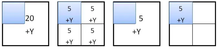
Fig. 1.Noise-added domain. (a) uniform non-partition. (b) uniform partition. (c) non-uniform non-partition. (d) non-uniform partition.
As shown in Fig 1, assume that (a) and (b) are uniformly distributed, (a) the noise is added to the area,(b) the noise is added after the area is partitioned. The numbers 5, 20 represent real statistics count for the area, +Y denotes the noise added to make this area satisfy differential privacy, and the blue district means the query area. Since the privacy budget is the same, the expected noise about two graphs (a) and (b) is the same. For the query result, (a) is (20+Y) / 4, and (b) is (5+Y). It is easy to see that the query error in the graph (b) is larger than in graph (a). However, for Figures (c) and (d), the query results are (5+Y) / 4 and (5+Y). Although Figure (c) reduces the noise error, it also increases the uni-form assumption error. So under normal circumstances, the noise error and the uniuni-form assumption error are opposite to each other. Utilizing the uniform assumption error esti-mate can reduce the noise error of the query result, but it will produce additional uniform assumption errors. However, subdivided regions can reduce the uniform assumption error of query results but increase the noise error. So how to balance the two kinds of errors in order to minimize the publishing error is a problem we need to discuss.
The methods described in the third section of this article all use tree structures to in-dex sensitive data. However, the tree structure does not involve the issue of minimizing publishing errors. Literature [8] proposed uniform grid (UG) and adaptive grid (AG) to minimize publishing errors. The publishing errors mainly include the added Laplace noise error and the uniform assumption error. UG and AG quantify the two parts of the error and get the grid partition density. The UG method partitions the spatial data set equally. However,we argue that the same partition method for sparse data and dense data will bring greater uniform assumption error. On that basis, the author proposes an AG method to adaptively partition the grid according to the data density. The disadvantage of the UG and AG methods is that the same privacy budget is allocated for sparse data and dense data whose effect on the noise error of them are different. Further consideration should be given to the adaptive allocation of privacy budgets based on data point density.
the other hand, the availability of published data(the similarity between original data and published data) is improved. We prove that the effectiveness of the algorithm is obtained in the experimental part compared with the relevant algorithm.
The rest of this paper is organized as follows: In section 2 we introduce the preliminar-ies and the related work. We propose our optimized algorithm for spatial decomposition and evaluate the algorithm compared with some of the previous ones in section 3 and 4. We conclude the paper in section 5.
2.
Related Work
Differential privacy was originally proposed in [4] to protect the results of queries. To pre-serve the privacy of individuals, Mechanisms must guarantee that the contribution of each individual for a query result cannot disclose data. We introduce the related technology in this paper in detail, including the notion of differential privacy and the data publishing method based on partition.
2.1. Differential Privacy Model
The main idea of the differential privacy protection model is to perturb the data by ran-dom noise before it is published. Hence, even if an attacker knows all the other record information except the target record, the individual user’s private information cannot be inferred through data mining and data analysis. In addition, differential privacy has a strict mathematical model, which can provide different degrees of privacy protection for data sets according to user requirements. This can protect users’ privacy information in various types of background knowledge attacks. Hence, the differential privacy protection model has been studied and perfected by scholars since its proposed, and gradually has a rigor-ous theoretical system [9]. Since differential privacy is defined on neighbor data sets, it is necessary for us to introduce the definition of neighboring data sets first.
Definition 1 (Neighboring data set) For two data setsD1andD2 with the same at-tribute structure,D1 andD2 are called neighboring data set, if and only if there is one different data record inD1andD2.
We give the definition of differential privacy based on the neighboring data set. Definition 2 (ε-differential privacy) A randomized algorithmA gives ε-differential privacy, for any pair of neighboring data setsD1andD2and for every set of outcomes O (O∈Range(A)),Asatisfies:
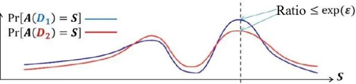
P r[A(D1) =O]≤eε·P r[A(D2) =O] (2) Theεin formula 2 is called privacy budget which represents the level of the privacy protection. The smaller theεis, the higher the protection level is. In order to make the results ofA(D1) andA(D2) have higher similarity, the data needs to be disturbed to a higher level, so the privacy protection level is improved and the availability of data is reduced [10]. On the contrary, the larger the value ofε, the less level of data disturbance will lead to better data availability, which may cause lower privacy protection. Nowadays, there is no good standard for the value ofε. Generally, the optimal value is constantly adjusted according to the level of privacy protection. It is always betweenln 2andln 5
The main idea of the differential privacy protection model is to hide the impact of a single data record on overall published data. It uses the idea of data perturbation to trans-form the single record by guaranteeing the invariance of the overall data on the probability to achieve the purpose of protecting the user’s private data. Figure 2 shows a statistical model of differential privacy, which illustrates the results of the privacy protection model implemented on a neighboring data set.
Fig. 2.Statistical Model of Differential Privacy
According to the definition of privacy we can know that it is used in data distribution mechanisms rather than directly applied to the data set. Intuitively, it can show that the behavior of differential privacy protection model on any two neighboring data sets are roughly the same in addition that the presence or absence of an individual does not affect the output of the algorithm. For example, there is a simplified medical record data set
D1 in which each record represents (name, diabetes), the second line is a boolean, 1 represents illness, and 0 represents no disease, as shown in Table 1. We assume that the opponent wants to know if Jack is sick or not and he also knows the number of rows in Jack’s database. Suppose the opponent’s query form isQi, which represents the sum of
the first I rows of theDiabetes. In order to know Jack’s prevalence, opponents perform queries Q5 (D1) and Q4 (D1) and then calculate their difference to know that Jack’s disease status corresponds to 1. This example shows that personal information may be affected even if no specific personal information is queried. If we construct the data set
D2by changing the last record to (Jack, 0) of table 1, the opponent can distinguish two neighboring data setsD1 andD2 by calculatingQ5-Q4. If the opponent gets the query valueQithrough ε-differential privacy, he cannot distinguish between two neighboring
data sets after selecting the appropriate value ofε.
Achieving differential privacy generally adopts two mechanisms: the Laplace mech-anism and the exponential mechmech-anism. These mechmech-anisms contains the definition of sen-sitivity. To make these definition understood easily, we give an introduction of global sensitivity [11].
Definition 3 (Global sensitivity) For a functionf :D→Rd, for any neighboring data
sets, the global sensitivity4f of functionfis defined:
4f = max
D1D2
||f(D1)−f(D2)||1 (3)
WhereD refers to the data set, Rd refers to d-dimensional vector,d is a positive
Table 1.Medical Dataset of Diabetic Patients
Name Diabetes
Ross 1
Bob 1
Phoebe 0
Carol 0
Jack 1
Global sensitivity represents the change in the output of the algorithm when changing any record in the data set.
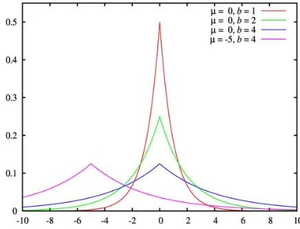
Laplace Mechanism The Laplace mechanism achieves differential privacy by adding noise that obeys the Laplace distribution to the original real query value. As shown in Figure 3, the probability density function of the Laplace distribution is:
f(x|µ, b) = 1 2b·e
−|x−µ|
b (4)
Whereµ is position parameter,brefers to scale parameter, whose value is up to 0. When the parameter changes, the Laplace probability distribution function changes as the Figure shows.
Definition 4 (Laplace mechanism) Given a functionf :D→Rdover a data set D, a
privacy budgetεand the global sensitivity4f,f satisfies Laplace mechanism when:
L(D) =f(D) +Lap(4f
ε ) (5)
WhereLap(λ)means the position parameter of Laplace distribution is 0, and the scale parameter isλ, same as 4εf.
A Laplace mechanism is used for the numeric query result [12]. We can add noise to the output value of original data set to affect the result of query to protect the data set. We can know that the smallerεcorresponding larger noise value according to taking different parameter values. The noise size of the Laplace mechanism needs to achieve a good balance between the protection level and practical application according to actual requirements [13].
Composition Theorems We need to consider the privacy budget of the entire process to be controlled withinε, because a complex privacy protection scenario often requires multiple applications of the differential privacy protection model. As a result, we need to apply the two composition theorem of the differential privacy protection model [14,15]
Definition 5 (Sequential composition)
Assume a set of algorithmsA1(D), A2(D), ..., An(D) whose privacy budgets are
ε1, ε2, ..., εnrespectively that satisfy differential privacy. For the data set D, a new
algo-rithmAcomposed of the above algorithmsA(A1(D), A2(D), ..., An(D)), givesPni=1εi
-differential privacy model. This theorem indicates that the privacy protection level of com-bined algorithms is the sum of all budgets in a differential privacy protection model se-quences [12].
Definition 6 (Parallel composition)
Assume a set of algorithmsA1(D), A2(D), ..., An(D) whose privacy budgets are
ε1, ε2, ..., εnrespectively that satisfy differential privacy. For the data set D which can be
partitioned into disjoint subcell data setsD1, D2, ..., Dn, a new algorithmAcomposed of
the above algorithmsA(A1(D), A2(D), ..., An(D)), givesmax(εi)-differential privacy
model.
In a differential privacy protection model sequences, the privacy protection level of combined algorithms is determined by the algorithm with the largest privacy budget, where the data sets input by each algorithm are disjoint. These two kinds of composi-tion theorems play an important role in the proof of the differential privacy proteccomposi-tion model algorithm. At the same time, the algorithm that satisfies differential privacy can also be partitioned into sub-algorithms, and then the sub-algorithm gets the correspond-ing privacy budget. For example, algorithmA’s privacy budget isε. IfAis divided into two processes,A1andA2, then privacy budgetεcan be divided intoε1andε2and then assigned toA1andA2respectively. We only need to makeA1 andA2meet the privacy protection levels ofε1andε2to satisfies differential privacy.
In addition,εrepresents the degree of privacy protection, so it is also important to choose appropriate allocate strategies. Common allocation strategies include linear allo-cation, uniform distribution, exponential alloallo-cation, adaptive alloallo-cation, and mixed strat-egy allocation [20].
The previous partition method is mainly divided into two categories: tree-based spa-tial decomposition and grid-based spaspa-tial decomposition. We will introduce these two methods in detail as follows [21].
2.2. Tree-Based Spatial Decomposition
The tree-based data distribution method is a method for hierarchically decomposing spa-tial data. The data points are partitioned into leaf nodes so that the leaf nodes can contain a small number of data points or a small data range. Non-leaf nodes represent the sum of the counts of children’s nodes. Unless otherwise specified, we assume that the tree structure is a complete binary tree that all root-to-leaf paths have the same length, and all internal nodes have the same output.
The tree-based data distribution methods can be roughly divided into two categories: data-independent partitioning and data-dependent partitioning. We define the data inde-pendent partitioning if the area is divided regardless of involving the basic data. On the contrary, when it is divided on the basis of the data, it is called the data-dependent parti-tioning, which may reveal data privacy [21].
Data-independent Tree Partitioning For the 2D spatial data, a representative exam-ple of the data-independent tree division is quadtree, which can be extended to high di-mensions named octree and other structures to represent data. Their feature is to set the partitioning method in advance and based on the attribute domain.
Data-dependent Tree Partitioning The representative structures of data-dependent tree structure are kd-tree and Hilbert R-trees which mainly depends on the input. We focus on the construction of kd-tree and the process of combining it with differential privacy.
The main construction process of kd-tree is divided into two steps:(1) select the dimensionkwith the largest variance in the k-dimensional data set, and then select the medianmin this dimension as the pivot to partition the data set to obtain two Subsets, while creating a tree node for storing the total calculated count values.(2)Repeat step
(1)for the two subsets until all subsets can no longer be divided. We store the data of the subset to the leaf node until it can’t be partitioned anymore [22].
The algorithm of using differential privacy based on kd-tree is called kd-standard [23]. Kd-standard’s privacy budget is divided into two parts: First, we need to determine the median value. The segmentation line may leak the true value of the median value if you do not use differential privacy to protect the segmentation process. Then we add Laplace noise to each level calculated count value of the kd-tree. Kd-standard may also have two problems with the above-mentioned quadtree: inconsistent query results and non-uniform allocation of privacy budgets. The solution is the same as a quadtree.
tree-dependent partitioning method in the previousl layer (lis set in advance). Then select the median with the maximum variance dimension as the pivot to divide recursively each time [24]. The rest of the tree uses a tree-independent partitioning method that sets up the partitioning process in advance. This algorithm makes the advantages and disadvan-tages of the two tree partitioning methods complementary, so the query results are more accurate.
2.3. Grid-Based Spatial Decomposition
In this section, we introduce the previous research achievements on the spatial data release and then gradually improve the method.
Uniform Grid Partition (UG) UG partitioning is a relatively simple way to partition the space. This method divides the data domain intom∗mequally sized grids, and then adds noise to a calculated count value for each grid, wheremis obtained by minimizing the sum of the noise error and the uniform assumption error. The disadvantage of UG parti-tioning is that all areas in the data set are treated equally where dense and sparse areas are partitioned in the same way. If there are fewer data points in a region, this method will result in the region being divided too much, which increases the noise error and hardly reduces the uniform assumption error. In addition, if an area is dense, uniform grid partition can make this area too rough, which in turn leads to large uniform assumption errors. Therefore, when the area is dense, a fine-grained partitioning method should be used because the uniform assumption error in this area far exceeds the noise error. Simi-larly, if a region is sparse, coarse-grained partitioning is used. To overcome this problem, researchers proposed Adaptive Grids (AG) partitioning based on the uniform grid method.
Adaptive Grid Partition (AG) The AG first performs uniform grid partition in a smaller granularity which is set asmax(10,14dN·ε
c e)since there is a second grid division, and
the privacy budget of the first layer isε1 =ε·α. Then, on the basis of the noise-added calculated count valueN of the first layer of the grid, the AG further adaptively selects the division granularity of the second layer grid. We find that AG improves the accuracy compared with UG obviously on the second layer.
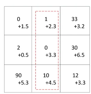
The advantage of AG partition method is that it can quantify two error sources on the basis of differential privacy to calculate the partition granularity. However, we find the drawback that AG does not adaptively allocate the privacy budget. According to the method proposed by Dwork [4], AG ignore the size of the query answer and add Laplace noise to each answer with the same scale parameters. The proposed method is more sus-ceptible to the amount of noise which may lead to a large relative errors especially when the calculated count value of the query is small. For example, Figure 4 shows a part area of the AG partitioning results: The two numbers in each grid are the original calculated count value and the added noise value, where the noise follows the Laplace distribution with the same scale parameters. For the dashed line area which represents the user’s query area, the corresponding noise added query result is21.1when the original query result is
Fig. 4.Example of Injecting Noise into Grid Partition
3.
Adaptive Grid-partitioning Noise Optimization Algorithm
In this section, we will introduce the improved algorithm in detail for the adaptive grid-partitioning. We introduced the quantification formulas for UG and AG, and illustrated their existing problems in related work. In that case, we proposed an optimized algorithm based on AG to solve these problems.
3.1. The Problem and Notions
The adaptive grid noise added publishing algorithm we proposed mainly addresses two aspects: (1) each grid adds Laplace noise with the same scale parameters (2) after the second-level grid is generated, the first level no longer provides useful information for the data set that may waste privacy budget. In response to the above problems, the cor-responding solutions are presented as follows: First, to avoid receiving a larger relative error when querying a very small value. we propose a method to reduce the relative error by adjusting the noise scale parameter of the counter value. Second, in order to save the first-level grid privacy budget, we generate the value in second-level grid by sampling from first-level grid noise calculated count value.
Before proposing the overall steps, we first introduce some parameters and the calcula-tion formula adjusted according to the differential privacy definicalcula-tion.G= [N1, ..., Nm1∗m1] is the set of count values for the first-level grid partitioning. Λ = [λ1, ..., λm1·m1] is a set of positive real numbers, corresponding to the noise scale parameterλi of each
Ni,(i∈[1, m1∗m1]).Y = [y1, ..., ym1∗m1]is a set of count values after adding noise to
Gin same scale parameter, whereyi =gi(G) +ηi andηiis sampled from the Laplace
distribution with scale parameteri(i∈[1, m1∗m1]).G0= [Y10, ..., Ym01∗m1]is the result of optimized noise added method after the use of adaptive noise adding algorithm.
The steps of the algorithm are as follows: In first step we perform a two-dimensional data set into first-level uniform grid partition with partition granularity
mi = max(10,14
q
N·ε
c ). The choice of the value cmainly depends on the uniformity
the grid setGgenerated in the first step to obtain the noise-added grid calculated count value setY. Next the grid sets to be optimized fromY are selected recursively and op-timized, where we use a noise optimization algorithm to satisfy the difference privacy guarantee in the meanwhile. It construct an optimized noise calculated count value set
G0. Finally we perform adaptive grid partition on the basis ofG0 with the granularity of
m2 = d
q
Y0·ε
2
c2 e, wherec2 =
c
2. The calculation process ofm2 andc2 are as follows: When the grid inG0is further divided into secondm2∗m2layer grids, only those queries whose query boundaries pass through the first layer grids are affected. These queries may contain0,1,2...m2−1rows (or columns) of the second-level grids, and therefore cor-respond to0,m2,2m2...(m2−1)m2 grids in second-level. When the query contains more than half of the second-level grid, the query is answered using Constraint Reason-ing, which uses the calculated count value of the first layer minus the calculated count value in the second-level grid that is not included in the query. Therefore, the query uses
an average of m1 2(
Pm2−1
i=0 min(i, m2−1))∗m2≈
m2 2
4 second-level grids, which means that the average noise error is approximate
q
m2 2 4 ∗
√ 2
ε2. In addition, the mean value of the uniform assumption error is approximately cY0
0∗m2. Finally, we minimize the sum of the average noise error and the uniform hypothesis error to get the minimum value ofm2is dqY0·ε
2
c2 e, wherec2=
c
2.
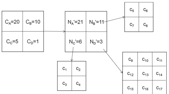
Fig. 5.Example of SGNO Partition (ε=0.5,α=0.5)
Figure 5 shows the partitioning process of SGNO, whereA,B,C, andDrepresent the four first-level grids. Constructing differential privacy SGNO requires three steps: First, calculate the partition granularity of the first-level grid, wherec = 10, and then add the Laplace noise with the scale parameter to the original values ofA,B,C, andDto obtain the noise calculated count valueN0. Secondly, we select the grid sets to be optimized from
N0 recursively using a noise optimization algorithm satisfying the differential privacy guarantee. The selected grid sets construct an optimized noise calculated count value set
calculate the granularity of the second-level grid on the basis ofG0, wherec2 = 5. We use the above formulas to obtain different partition granularity for different noise-added count valuesN0, and add Laplace noise with scale parameter to each second-level grid. Finally, SGNO structure is published with noise count.
3.2. Noise Optimized Partitioning
The principle of the NOP (Noise Optimization Partitioning) [16] is to add a uniform scale parameterλi(1 ≤i ≤ mi∗mi)to the second layer of the grid to obtain a set of
noise-added countsY, and then adjust the noise scale parameter setΛ= [λ1, ..., λm1∗m1] continuously under the constraint of differential privacy to generate updated set of noise countY0. The key question of this algorithm is whetherY0is to add noise to the original valueNi(1≤i≤mi∗mi)through a new set of scale parameters, or to adjust the noise
value set to generateY0on the basis ofY, so next we consider for both cases separately. If the first and the second level of the grid noise adding process are independent, then the total privacy budget is2/λ+2/λ0, where the privacy budget of the second layer grid is
2/λ0. However, the result of the first level grid partitioning is useless after the generating of the second layer grid, which means the privacy budget used by the first level grid is wasted. To solve the above problems, we argue that the noise-added value of the second level grid obeys Laplace distribution and is sampled from the distribution that depends on the first level grid, which can save part of the privacy budget.
We use formula derivation to explain the process of reducing the privacy budget: First, for the data setT1, the first layer of partitioning produces a result ofY, and the second produces a result ofY0.Y’s result is useless afterY0is generated which can quantify as the following formula:
P r[T =T1|Y =y, Y0=y0] =P r[T =T1|Y0 =y0] (6) Formula 6 allows us to use the privacy budget more efficiently. When Equation 6 is satisfied, we can apply the Bayesian equation twice to derive the following derivation for two neighbor data setsT1andT2:
P r[Y0=y0, Y =y|T =Ti]
=P r[T =Ti|Y0=y0, Y =y]·
P r[Y0=y0, Y =y]
P r[T =Ti]
=P r[T =Ti,|Y0 =y0]·
P r[Y0 =y0, Y =y]
P r[T =Ti]
=P r[Y
0=y0|T =T
i]P r[T =Ti]
P r[Y0=y0] ·
P r[Y0=y0, Y =y]
P r[T =Ti]
=P r[Y0=y0|T =Ti]·P r[Y =y, Y0 =y0]
(7)
distribution with the positional parameterq(T)and the scale parameterλ0. Second, it is dependent on Y. Equation 6 and 7 get the following derivation process:
P r[Y0=y0, Y =y|T =T1]
P r[Y0=y0, Y =y|T =T 2]
=P r[Y
0=y0|T =T
1]·P r[Y =y|Y =y0]
P r[Y0=y0|T =T
2]·P r[Y =y|Y =y0]
=P r[Y
0=y0|T =T 1]
P r[Y0=y0|T =T 2]
≤exp(2/λ0)
(8)
From equation 8 we can get an upper bound of the privacy budget. which means we can achieveY0on the basis ofY. The total privacy budget is only2/λ0to ensure no pri-vacy budget is wasted onY.
From the above process, we learned that ifY obeys the Laplace distribution and sam-ples from theY-dependent distribution, it can save some privacy overhead. So we define the conditional probability distribution function forY as follows:
fµ,λ,λ0(y0|Y =y) =λ
λ0
·
exp(−|y0 −µ|
λ0 )
exp(−|y−µ|
λ )
·γ(λ0, λ, y0, y)
γ(λ0, λ, y0, y) = 1 4λ
· 1
cosh( 1
λ0)−1
·(2 cosh(1
λ0·exp(− |y−y0 |
λ )
−exp(−|y−y0 −1|
λ )
−exp(−|y−y 0+ 1|
λ ))
(9) The probability density function ofY0 can be further obtained from the conditional probability density function. Whenµ≤y,ξ= min{µ, y−1}. We can obtain the follow-ing formula accordfollow-ing to the conditional probability density function fory0≤ξ.
f(y0) =ey
0/λ0
·γ(λ0, λ, y0, y)· λ
λ0·exp( −µ
λ0 +
y−µ λ )
γ(λ0, λ, y0, y) =ey0/λ· 1
4λ
· 1
cosh( 1
λ0)−1
·(2 cosh(1
λ0
·exp(−−y
λ
)−exp(−1−y
λ
)−exp(−−1−y
λ
)) (10)
Formula 7 can be simplified asf(y0)∝exp(y0/λ+y0/λ0), meanwhile, we can obtain
y0∈(ξ, y−1],f(y0)∝exp(y0/λ−y0/λ0)andy0∈(y+ 1,+∞],f(y0)∝exp(−y0/λ−
y0/λ0). Based on this, the random variablesθ1, θ2, θ3that follow the probability density functionfcan be calculated and their formula is as follows:
θ1=
Z ξ
−∞
f(y0)dy0
=λ·(cosh(
1
λ0)−cosh(
1
λ)·exp(
1
λ0 +
1
λ)·(ξ−µ))
2(λ0+λ)·(cosh(1
λ0)−1)
(11)
θ2=
Z y−1
ξ
f(y0)dy0
=λ·(cosh(
1
λ0))·(e
1
λ0 −eλ1)·(1−e−
1
λ0−λ1)
4(λ−λ0)·(cosh(1
λ0)−1)
·(1−exp((1
λ0 −
1
λ)·(ξ−y+ 1))
θ3=
Z +∞
y+1
f(y0)dy0
=λ·(cosh(
1
λ0)−cosh(
1
λ)·exp( µ−y−1
λ0 −
µ−y+1
λ ))
2(λ0+λ)·(cosh(1
λ0)−1)
(13)
For the remaining space(y−1, y+ 1), we obtain its probability density function through the standard importance sampling function. We will introduce the specific process in the algorithm. The formula ofϕin the algorithm1is as follows:
ϕ= 1
2λ0 ·
cosh(λ10)−exp (−
1
λ)
cosh(λ10 −1)
·exp (y−µ
λ −
max{0, y−µ−1}
λ0 ) (14)
The algorithm 1 represents a specific process of NOP, where the input is original cal-culated count valueµ, a noise-added calculated count valuey, an original scale parameter
λ, and an adjusted scale parameterλ0, and the output is an updatedy.
3.3. Self-adaptive Grid-partitioning Noise Optimization Algorithm
We use the algorithm2to describe the grid-based adaptive noise-added publishing method in detail. The pseudocode of this algorithm is shown in Algorithm 2. The input of the al-gorithm is data setT, privacy budgetε, initial privacy budgetλmax, and privacy budget
varianceλ∆. The output is Adaptive Grid AG. The algorithm first averages the data set to
get a uniform grid set UG and an original privacy setΛ. Then the grid to be optimized is selected recursively from the UG. We adjust the scale parameters and complete the noise optimization process with former algorithm. If this process does not satisfy the differen-tial privacy, the changes made to the noise scale parameters are restored. Finally, AG is adaptively partitioned with the updated UG set.
We need to explain the process of selecting the grid to be optimized. Ideally, run-ning a noise optimization algorithm on a selected set of grids may reduce the overall more error and make slightly lower privacy overhead, so the criteria for PickQueries function selection grids is to maximize the ratio between the value of overall error re-duction and privacy budget increase value. First, calculate the privacy budget increase value. Each grid has the same scale parameter λi(i ∈ [1, m1 ∗m1]) at first with the global sensitivityg1=Pi∈[1,m1∗m1]
2
λi. Then we use the noise optimized algorithm for
the selected j−thgrid, and the corresponding global sensitivity is changed to g2 = 2
λj−λ∆ +
P
i∈[1,m1∗m1]∧i6=j 2
λi, the privacy budget applied by the noise optimized
algo-rithm is g2−g1 = λ 2
j−λ∆ −
2
λj. Second, we calculate the total error reduction value.
The relative error of each grid is λi
max{yi,δ}(i ∈ [1, m1∗m1]). Then, the relative error
of grid UG isP
i∈[1,m1∗m1]
λi
max{yi,δ}. After applying the noise optimized algorithm, the
total relative error becomes λj−λ∆
max{yi,δ}+
P
i∈[1,m1∗m1]∧i6=j
λi
max{yi,δ}, and the change of
total relative error is obtained to 2λj−λ∆
max{yi,δ}, so that the average relative error variation is
1
m1·m1 ·
2λj−λ∆
max{yi,δ}. Therefore, the ratio between the overall error reduction value and the
privacy budget increase value ism1 1·m1·
2λj−λ∆
max{yi,δ}/(
2
λj−λ∆−
2
λj). So we choose the grid
Algorithm 1: NOP (µ, y, λ,λ0)
Input:µ, y, λ, λ0 1
Output:y 2
Initial:mark=true 3
ifµ > ythen 4
µ=-µ,y=-y 5
mark=f alse 6
ξ= min{µ, y−1} 7
generate a random variable u uniformly distributed in[0,1]
8
ifµ∈[0, θ1]then
9
f(y0)∝exp(y0/λ+y0/λ0) //y’is a random variable generated f rom(−∞, ξ];
10
else 11
ifµ∈[θ1, θ1+θ2]then
12
f(y0)∝ 13
exp(y0/λ0−y0/λ) //y’is a random variable generated f rom(ξ, y−1];
else 14
ifµ∈[1−θ3,1]then
15
f(y0)∝exp(−y0/λ− 16
y0/λ0) //y’is a random variable generated f rom(y+ 1,∞);
else 17
whiletruedo 18
generate a random variabley0uniformly distributed in (y-1,y+1)
19
generate a random variableµ0uniformly distributed in [0,1]
20
ifµ0≤f(y0)/ϕthen 21
break;
22
ifmark=truethen 23
returny0 24
else 25
return−y0 26
3.4. Privacy Analysis
Algorithm 2:SGN O(T, N, δ, ε, λmax, λ∆, α)
Input:Dataset T,the sanity bound δ,privacy budget ε,constant λmax, λ∆, 1
Output:Adaptive Grids AG 2
Initial:let T be partitioned unif ormly with m1 = max(10,14dN εc e)
3
let m=m1∗m1and gibe the i−th(i∈[1, m,])grid in U G 4
initialize Λ= [λ1, ..., λm1·m1], such that λi=λmax
5
ifGS(U G, Λ)> εthen 6
return∅ 7
Y =LaplaceN oise(U G, Λ) //Add Laplace noise to every grid in U G 8
Let U G0=U G 9
whileU G06=∅do 10
U∆=P ickQuries(U G0, Y, Λ, δ) 11
fori f rom1to mdo 12
ifgi∈U∆then 13
λi=λi-λ∆ 14
ifGS(U G, Λ)≤εthen 15
fori f rom1to mdo 16
ifgi∈U∆then 17
yi=N OP(gi, yi, λi+λ∆, λi) 18
else 19
fori f rom1to mdo 20
ifgi∈U∆then 21
λi=λi+λ∆ 22
U G0=U G\U∆ 23
U pdate U G by Y 24
let U G be partitioned by m2=dY
0(1−α)ε
C2 eto get AG
25
ReturnAG;
26
4.
Evaluation
In this section we compare the effectiveness of the algorithm proposed in section 4 with some previous methods. We introduce the process and results in detail.
4.1. Environment
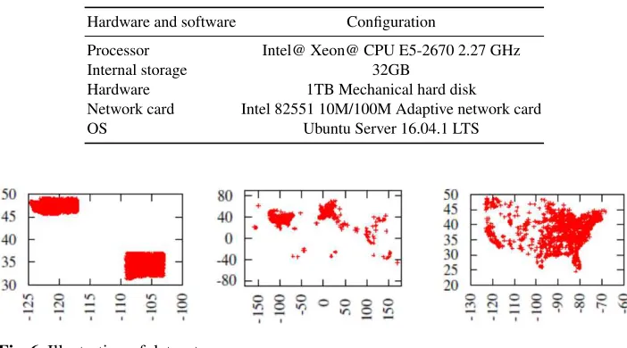
Experiment Platform Table 2 shows the relevant configuration information of the ex-periment platform. We have implemented the encoding algorithm proposed in section 4 in the Linux operating system.
Table 2.Configuration of Experiment Platform
Hardware and software Configuration
Processor Intel@ Xeon@ CPU E5-2670 2.27 GHz
Internal storage 32GB
Hardware 1TB Mechanical hard disk
Network card Intel 82551 10M/100M Adaptive network card
OS Ubuntu Server 16.04.1 LTS
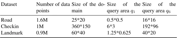
Fig. 6.Illustration of datasets
In order to verify our proposed grid-based adaptive noise-added publishing algorithm, we used three datasets shown in Figure 6.
(1)Road: This data set consists of the GPS coordinates of road intersections in Wash-ington State and New Mexico and is derived from the2006U.S. census data in the TIGER/ Line data set. There are approximately1.6million data points in the data set, roughly cor-responding to human activities. As shown in the first picture of Figure6, the distribution of data points is somewhat special. Two data points are dense where is distributed in two states, and almost no data points in there.
(2)Checkin: This data set consist of the check-in data of the location-based social net-work Gowalla which records the time and location of the user’s check-in from February
2009to October2010. We use the location information for evalution. There are approxi-mately one million data points in the data set. As shown in the second picture of Figure
6, the data distribution is sparse.
(3)Landmark: This data set contains information on the location of landmarks such as schools, post offices, shopping malls, construction sites, and train stations in48states in the United States. It originated from the2010Census TIGER. The data set contains approximately900,000 data points. As shown in the third picture of Figure6, the data distribution is relatively uniform.
Table3gives the detailed information of the three data sets, including the number of data points, the size of the domain, and the size of the query area used in the evaluation of the experiment, whereq1is the smallest query area andq6is the largest query area.
Table 3.Information on Datasets
Dataset Number of data points
Size of the do-main
Size of the query areaq1
Size of the query areaq6
Road 1.6M 25*20 0.5*0.5 16*16
Checkin 1M 360*150 6*3 192*96
Landmark 0.9M 60*40 1.25*0.625 40*20
the mixed-tree partitioning algorithm [22] which belongs to the same general-distributed class publishing algorithm to verify the effectiveness of the grid-partitioning algorithm.
Evaluation Metrics The differential privacy protection mechanism is mainly obtained by adding noise to the original calculated count value. This mechanism has two purposes. On one hand, it should to protect the privacy of each user. On the other hand, it should obtain that the published results will be still usable. Therefore, we quantify these two as-pects through various index parameters, hoping to reach a balance.
For grid-based spatial data publishing algorithms, we measure the accuracy of pub-lished data by calculating relative errors.
For a queryr, we useA(r)to represent the correct answer forr. For the methodM
and a queryr, we use to represent the queryrwhich is answered using an index structure constructed by the methodM. The formula for the relative error is:
REM(r) =
|QM(r)−A(r)|
max{A(r), ρ} (15)
where the queryrhas6kinds of sizes,q1 is the smallest, and the length and width ofqi+1 are respectively increased by2 times on the basis ofqi, andq6is maximal and covers1/4to1/2of the entire space. The specific information is shown in Table3. We randomly generate200queries for each query size and calculate their relative errors.
ρis set to0.001|D|, whereDrepresents the total number of data points in the data set. The reason why we maximize the denominator is to preventA(r) = 0. When the query
ris medium in size,REM(r)tends to be the largest. When the query is large, it may be
small becauseA(r)is large.
4.2. Evaluation
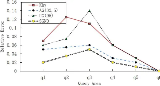
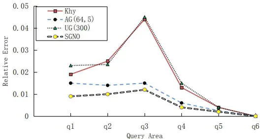
We proposed a grid-based spatial partitioning data publishing algorithm for publishing geo-spatial data based on a differential privacy protection model. In the experimental re-sults,Khy represents the kd-hybrid algorithm proposed in [24], UG represents uniform
ε= 0.1, the first level of the AG method divides the granularity of the reference [26] rec-ommended value of the experiment, which means the granularity of the Road, Checkin, and Landmark data sets is 16, 32, and 32 respectively. Whenε= 0.1, the granularity of the Road, Checkin, and Landmark data sets is32,64, and64respectively. UG and AG take the correspondingc = 10,c2 = 5,β = 0.5, in the granularity formula. Figure7to Figure12give the average curve of the relative error of the random query region for the four algorithms on the three data sets when the value ofεis0.1or1respectively. In order to make the experimental results more general, we will run the four algorithms50times, and finally take the average of them.
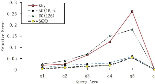
Fig. 7.Experiment Result on Dataset Road withε= 0.1
Fig. 9.Experiment Result on Dataset Checkin withε= 0.1
Fig. 10.Experiment Result on Dataset Checkin withε= 1
Fig. 12.Experiment Result on Dataset Landmark withε= 1
Figure7 and Figure 8 show the experimental results for the data set Road at ε = 0.1andε = 1respectively. It can be seen that the relative error of the four algorithms increases with the increase of the query area, and the relative error at the queryq5reaches the maximum, atq6 decreases sharply and is almost close to zero. The reason for this trend is that the query areaq6occupies between1/4and1/2 of the entire query space, making the true answer value large, thus the relative error is small.
Whenε = 0.1, the relative errors of the first four queries of kd-hybird and UG are relatively close, but the kd-hybird changes more greatly in the latter two queries. The AG and our method SGNO are superior to kd-hybird and UG on any query. The relative error of the first four queries of SGNO is better than AG, and the query result ofq5 is close to AG. The reason is that when the query range is relatively large, the actual query value is also relatively large, which makes the effect of noise optimization cannot be clearly displayed. Whenε= 1, the relative error of the corresponding four algorithms is reduced since the degree of privacy protection is reduced thus the amount of added noise is reduced too.
Figure9 and Figure10show the experimental results of the data set Checkin when
ε= 0.1andε= 1respectively. It can be seen that the relative error of the four algorithms increases with the increase of the query area, and the relative error at the queryq4reaches a maximum when decreasing sharply atq5andq6.
Whenε= 0.1, the results of kd-hybrid and UG are mostly similar. The overall trend of UG and SGNO is relatively close, but the relative error of SGNO is generally lower than AG, especially when the query area is relatively small. The reason is that SGNO optimizes the amount of noise added in each grid. In that case, we reduce the relative error of each grid so the entire error is improved. However, when the query area is relatively large, the real calculated count value is relatively large, making the optimization effect difficult to show. Whenε= 1, kd-hybrid and UG results change more drastically. Figure
11and Figure12show the results of the Landmark data sets whenε = 0.1andε = 1
ε = 0.1 andε = 1, the overall trend of UG and SGNO is relatively close. SGNO is mostly better than the other three algorithms.
From the figure, we can observe our SGNO methods have performed better than other methods. The performance of the UG method is similar to that of the kd-hybrid method. Above all, the results of SGNO in most queries are better than the other three algorithms.
5.
Conclusion
This article is based on application scenarios for the partition based data distribution algo-rithm. For the partition-based data distribution method, we first uniformly partitions the original spatial data, add a Laplace noise with uniform scale parameters, and then select the set of grids to be optimized in a standard way that is based on the maximum ratio between the value of overall error reduction and privacy budget increase value, then op-erate noise optimized algorithm for the grid. This process is recursive until all grids have been optimized. This grid-based self-adaptive noise-added publishing algorithm solves the problem of the noise scale parameters added uniformly to each grid and the waste of the first-level grid privacy budget.
At the same time, for the above differential privacy data publishing algorithm, prob-lem how to support dynamic data partitioning is the future research direction.
Acknowledgements Supported by the Double-class Construction Innovation Project 014-3190518. Supported by the National Nature Science Foundation of China 61370198, 61370199, 61672379 and 61300187. Supported by the Liaoning Provincial Natural Sci-ence Foundation of China NO. 2019-MS-028.
References
1. Xiong, P., Zhu, T. Q., Meng, X. F.: A Survey on Differential Privacy and Applications, Chinese Journal of Computers, 37(1), 101-120.(2014)
2. Gherari, M., Amirat, A., Laouar, R., Oussalah, M.: A smart mobile cloud environment for modelling and simulation of mobile cloud applications, International Journal of Embedded Systems, 9(5), 426-443.(2017)
3. Chen, P., Chen, J., Huang, J.: Multi-user location-dependent skyline query based on dominance graph, International Journal of Computational Science and Engineering, 13(3), 209-218.(2016) 4. Dwork, C.: Differential privacy[J], Lecture Notes in Computer Science, 26(2), 1-12.(2006) 5. Li, N., Li, T., Venkatasubramanian, S.: T-closeness: privacy beyond k-anonymity and
l-diversity[C], Proceeding of the IEEE 23rd International Conference on Data Engineering (ICDE), 106-115.(2007)
6. Cormode, G., Procopiuc, C., Srivastava, D., Shen, E., Yu, T.: Differential private spatial de-compositions, IEEE International Conference on Data Engineering (ICDE), 20-31.(2012) 7. Zhang, X. J., Meng, X. F., Chen, R.: Differentially Private Set-Valued Data Release against
In-cremental Updates, International Conference on Database Systems for Advanced Applications, 392-406.(2013)
8. Qardaji, W., Yang, W., Li, N.: Differentially private grids for geospatial data[C], Proceedings of IEEE 29th International Conference on Data Engineering (ICDE), 757-768.(2012) 9. Ebadi, H., Sands, D., Schneider, G.: Differential privacy: now it’s getting personal[C],
10. Gruska, D. P.: Differential privacy and security[J], Fundamenta Infomaticae, 143(1), 73-87.(2016)
11. Dwork, C., McSherry, F., Nissim, K. et al.: Calibrating noise to sensitivity in private data anal-ysis, Theory of Cryptography, 265-284.(2006)
12. Mcsherry, F., Talwar, K.: Mechanism design via differential privacy, IEEE Symposium on Foundations of Computer Science, 94-103.(2007)
13. Geng, Q., Viswanath, P.: The optimal noise-adding mechanism in differential privacy, IEEE Transactions on Information Theory, 62(2), 925-951.(2016)
14. Kairouz, P., Oh, S., Viswanath, P.: The composition theorem for differential privacy, Proceed-ings of the 32nd International Conference on Machine Learning, 63(6), 4037-4049.(2015) 15. Mcsherry, F. D., Meng, X. F.: Privacy integrated queries: an extensible platform for
privacy-preserving data analysis, Communications of the ACM, 53(9), 89-97.(2015)
16. Xiao, XX., Bender, G., Hay, H. et al.: iReduct:differential privacy with reduced relative errors, ACM SIGMOD International Conference on Management of Data, 229-240.(2011)
17. Li, Y. D., Zhang, Z., Winslett, M. et al.: Compressive mechanism:utilizing sparse representa-tion in differential privacy, Proceedings of the 10th Annual ACM Workshop on Privacy in the Electronic Society(WPES), 177-182.(2011)
18. Peng, S., Yang, Y., Zhang, Z. et al.: DP-tree:indexing multi-dimensional data under differential privacy, Proceedings of the 2012 ACM SIGMOD International Conference on Management of Data, 864-864.(2012)
19. Hardt, M., Talwar, K.: On the geometry of differential Privacy, Proceedings of the 42nd Annual ACM Symposium on Theory of Computing(STOC), 705-714.(2010)
20. Zhang, X. L., Wu, Y. J., Wang, X. D.: Differential Privacy Data Release through Adding Noise on Average ValuE, International Conference on Network and System Security, 37(1), 417-429.(2012)
21. Dwork, C.: Differential privacy: a Survey of results, International Conference on Theory and Applications of MODELS of Computation, 1-19.(2008)
22. Cormode, G., Procopiuc, C., Srivastava, D. et al.: Differentially private spatial decompositions, Proceedings of IEEE 28th International Conference on Data Engineering (ICDE), 41(4), 21-31.(2011)
23. Kamel, I., Faloutsos, C.: Hilbert R-tree: an improved R-tree using fractals, International Con-ference on Very Large Data Bases, 500-509.(1994)
24. Roy, I., Setty, S. T. V., Kilzer, A. et al.: Airavat: security and privacy for MapReduce, Pro-ceedings of the 7th USENIX Symposium on Networked Systems Design and Implementa-tion(NSDI), 297-312.(2010)
25. Machanavajjhala, A., Kifer, D., Gehrke, J. et al.: L-diversity: privacy beyond k-anonymity, ACM Transactions on Knowledge Discovery from Data(TKDD), 1(1), 3-14.(2007)
26. Xiao, Y., Xiong, L., Yuan, C.: Differentially private data release through multidimensional partitioning, Proceedings of the 7th VLDB Workshop on Secure Data Management (SDM), 150-168.(2011)
Haoze Lv is currently in school with the Department of Computer Science in Dalian Maritime University. His research mainly focuses on Big data and privacy protection.
Minghui Liis currently pursuing the master’s degree with the Department of Computer Science in Dalian Maritime University. Her research mainly focuses on Big data and privacy protection.
Zhiyang Li(corresponding author) is currently an associate professor at the Information Science and Technology College, Dalian Maritime University, China. He received the Ph.D. degree in computation mathematics from Dalian University of Technology, China in 2011. His research interests include computer vision, cloud computing and data mining.
Zhiyi Huangreceived the BSc degree in 1986 and the PhD degree in 1992 in computer science from the National University of Defense Technology (NUDT) in China. He is an Associate Professor at the Department of Computer Science, University of Otago. He was a visiting professor at EPFL and Tsinghua University in 2005, a visiting scientist at MIT CSAIL in 2009, and a visiting professor at Shanghai Jiao Tong University in 2013. His research fields include parallel/distributed computing, multicore architectures, operating systems, green computing, cluster/grid/cloud computing, high-performance computing, and computer networks. He has more than 130 publications in peer-reviewed conferences and journals, many of which are top ranked.