RESEARCHARTICLE
A Graph-Based Semi-supervised
Approach to Classification Learning
in Digital Geographies
Pengyuan Liu and Stefano De Sabbata
School of Geography, Geology and Environment, University of Leicester, United Kingdom
June 26, 2020
Abstract: As social media have become an integral part of many people’s everyday life, there has been an increasing interest in exploring how the content shared through those on-line platforms comes to contribute to the collaborative creation of places in physical space. Indeed, the distinction between online and physical spaces is rapidly degrading. However, exploring those digital geographies is a complex task due to the quantity and variety of data. In this paper, we introduce a semi-supervised, deep neural network approach to classify geo-located social media posts based on their textual and visual content, as well as geographical and temporal aspects, using a limited set of customisable categories. Our innovative approach is rooted in our understanding of social media posts as augmenta-tions of the time-space configuraaugmenta-tions that places are, and it comprises a stacked multi-modal autoencoder neural network to create joint representations of text and images, and a spatio-temporal graph convolution neural network for semi-supervised classification. The results presented in this paper show that our approach performs the classification of social media content with higher accuracy than traditional machine learning models as well as two state-of-art deep learning frameworks. Thus, the presented approach has the poten-tial to develop into a powerful tool to complement content analysis in the study of digital geographies.
1
Introduction
Social media have become major platforms for people to communicate and exchange infor-mation regarding a wide range of topics. Despite the unequal geographies of social media platforms [9], there is a growing interest in analysing such information from a geographic perspective within the field of digital geographies [6]. However, traditional qualitative analysis often struggles with tackling large datasets, and the volume of data produced daily on social media is enormous. Thus quantitative analysis and summarisation are frequently necessary steps in digital geographies. That creates a strong association with GIScience, where data mining approaches have been applied to identify users’ opinions and online trends, to study the emergence of place from space through content production [25], or to monitor events from football to earthquakes [21, 32, 50, 63] and to understand the digital representations of a place [8].
In computer science and related disciplines, sentence-level topic extraction from social media posts has attracted wide attention, where research has mainly focused on super-vised learning approaches with well labelled and balanced data [44]. However, labelling large volumes of social media posts can be a lengthy and costly procedure as it requires a significant amount of human intervention. Such approaches are only viable when a pre-defined set of topics or categories has been agreed upon by a large number of stakeholders, for instance, for monitoring scheduled events or natural disasters. Such approaches are more difficult to employ effectively for exploratory analysis or monitoring of unexpected events. So far, limited attention has been given to the study of exploratory analysis, where only vague or no categories at all have been pre-defined. Conversely, semi-supervised learning approaches, which do not require complete labelled training, have achieved com-petitive results in learning accuracy, without the time and costs needed for the training data preparation step of supervised learning [65]. However, there are severe concerns about the uncertainties of social media analysis, as raw data collected from social media platforms tend to be noisy and fuzzy, rendering any approach problematic when applied to “live” data [52]. Thus, creating a robust framework, able to produce consistent results with im-balanced datasets is a crucial task in digital geographies.
In this paper, we present and test an approach to the exploratory analysis of social media content capable of classifying posts based not only on the textual component but also taking into account their visual content. The latter is a crucial contribution of our approach, as only a handful of papers account for images when conducting quantitative analyses of social media content [23, 31, 60]. Furthermore, conceptualising posts as “augmentations” [25] of places, understood as “time-space configurations” [3], we go beyond the geotag [17] by developing graph convolutional networks that account for the relationships between each post and its spatio-temporal neighbours. To the best of our knowledge, the proposed model is the first to account for all four aspects (text and media, as well as geographical and temporal information) using a deep learning approach.
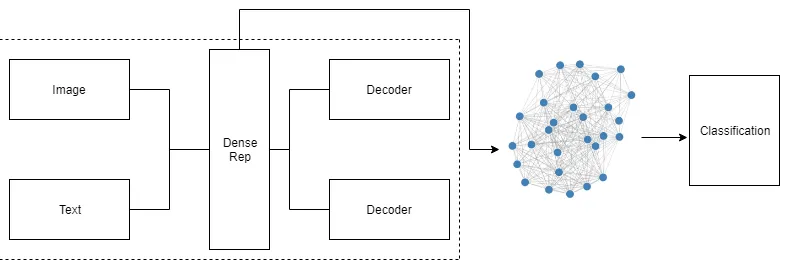
Our approach thus comprises two main components. The first component is a stacked multi-modal autoencoder developed in our previous work [39], which is used to create dense representations of text and image content. The second component extend our pre-vious spatial graph convolutional network [38] into a spatio-temporal graph convolutional network, which encodes the geographical and temporal proximity relationship between social media posts.
1. we explore effects of including spatio-temporal aspects using a graph convolutional network on the classification of social media posts;
2. we provide a robust and detailed comparisons between different set-ups of our pro-posed framework and other deep learning approaches;
3. we explore the effects of imbalanced datasets on the classification accuracy and eval-uate how data uncertainty (e.g., variations in the number of cases in each category) affects the classification results.
2
Related Work
Due to the potential of social media platforms for exploring human activities in space and the narrative of places [1], social media platforms in general, and Twitter in particular, have been at the centre of data-driven analysis in GIScience and quantitative geography for about a decade [45] from location mining to residence location prediction [2, 19, 49]. Lee et al. [37] proposed a geo-social event detection system to detect unusual regional social ac-tivities based on geo-tagged Twitter messages, and identified a strong point of connection between local events and crowd behaviours detected from posts shared on the platform. Tsou et al. [53] showed the effectiveness of using combined content from tweets and multi-ple web sources to identify relevant spatial and temporal patterns regarding specific events. Studies by Longley and Adnan [40] and Wakamiya et al. [54] also illustrate how the spatial analysis of social media progresses our understandings of socio-spatial patterns and crowd behaviour within cities.
Despite the growing popularity of visual content in social media, limited work has been done so far on such content within the field of GIScience. This is a severe limitation, as image content is a key component of social media posts – especially considering the rise of image-focused platforms such as Instagram or Flickr. According to a recent survey1,
images or photos constitute around 36% of posts on Twitter, which renders the analysis of visual data an interesting area to explore. Visual content can also provide rich infor-mation regarding places, the use of space, and people’s experiences of landscape. Earlier work on visual content of geo-located media mostly focused on tags or meta-data. For in-stance, Hollenstein and Purves [28] investigated the use of geo-located photos from Flickr that users have tagged with keywords such as “downtown” or “citycentre” to explore a user-defined centre of a city. Panteras et al. [48] developed a social multi-media triangu-lation process to identify natural disasters using Twitter text content and Flicker image meta-data. With the help from the rising methodologies of traditional machine learning, Gao et al. [23] proposed a method for geo-located event detection from micro-blogs, they generated an intermediate semantic entity, named micro-blog clique (MC) based on text similarities, image similarities, location similarities and temporal similarities to explore the highly correlated information among the noisy and short micro-blogs. Xu et al. [60] intro-duced their framework to detect urban emergency events based on the correlations among images, texts and locations. Previous research mainly focus on using traditional machine training approaches based on low- or mid-level attributes from texts and images – e.g., td-idf for text representation, spatial pyramid image features for image representation.
Current developments in deep learning technologies open new opportunities for bridg-ing the gap, and movbridg-ing beyond the use of tags chosen by the users and low- or
level attributes, and combine high-level representations extracted directly from the visual content (e.g., images). Within the discipline of computer science, some work [22, 59, 62] has been devoted to using convolutional neural network to analyze users’ sentiment directly from the images posted on social media posts. Attracted by the growing popularity of multi-media content on social media posts, research has been widely conducted from uni-modal analysis to multi-media content study. For example, Cai and Xia [11] proposed a framework using two separate convolutional neural network (CNN) to extract represen-tations from text and images from tweets, and feed them in to another CNN to predict sentiment on Twitter multi-media content. Chen et al. [14] trained separated classifiers for images and text simultaneously, and proposed a weighted co-training approach for the joint visual-textual sentiment analysis. Mouzannar et al. [46] combined multiple pretrained convolutional neural networks that extract representations from raw text and images inde-pendently, and classify them to identify damage related information. Huang et al. [30] pro-posed a framework based on Deep Canonical Correlation Analysis [5] to jointly learning representations from text and image, and further identify event-related tweets.
To out best knowledge, within the discipline of GIScience, apart from the work we pre-sented [39], Huang et al. [31] are the only other authors to apply this technology on text and images to analyse geo-located social media posts. Huang et al. [31] proposed an end-to-end fully supervised framework to report geo-located flood events using Twitter posts. They adopted two convolutional neural network architectures to extract representations from texts and images, and combine both representations for filtering out flood-related tweets from a massive tweets pool. However, their approach focuses on a binary classification and does not account for the geo-location of social media post in the context of the classification.
3
Research Questions
Based on the literature review discussed above, we propose the following research ques-tions:
1. How can we combine information extracted from multimedia content (text and im-ages) from social media data to better understand social media posts?
2. How can the spatial component of social media posts benefit the semantic categoriza-tion of their contents?
3. How can the temporal component of social media posts further improve the semantic categorization of their contents?
In the reminder of this paper, we propose a deep learning framework to explore the above research questions, and a series of experiments to test it.
4
Case study
Twitter API2. The geo-located tweets we retrieved from Twitter contain both image and
text, and precise geographic coordinates. In order to filter bots, we limited the overall amount of tweets per account to 365. The final dataset has 16,950 tweets, which clearly wouldn’t be easy to analyze manually, in a tweet-by-tweet manner.
In digital geographies studies, it is common to explore a sample of a few hundred tweets, and conduct content and visual analysis by categorizing the sampled tweets through a relatively small number of “codes” (i.e., labels – see, e.g., [7, 20]).
In this scenario, the proposed approach described in the next section (Section 5) would be able to learn the labels from the sample and deploy the same categorization to the whole dataset. The labeled dataset could then be used for further exploration of the specific topics. For the scope of this paper, we randomly sampled 701 tweets from the dataset, that have been manually labeled as discussed below.
4.1
Labeling
We manually labeled the randomly sampled 701 tweets into 11 different categories: Ani-mals, Entertainment, Food, Nature, News, Personal, Places and attractions, Social, Sports, Work and Not informative. The latter category includes advertisement and other content that was difficult to interpret. The category Personal includes content related to personal daily activities such as shopping or selfies, whereas tweets in the category Social are related to social activities (e.g., parities). The category Work mostly contains tweets related to of-fices environment or the description of users’ work. As illustrated in Figure 1, the sampled dataset is unbalanced as certain categories are more represented than other, for instance, there are 166 tweets regarding Places and attractions while only 8 tweets in the category Animals.
It is important to emphasis that we labeled our social media only based on their text and image content rather than labeling them based on their location or geographic content explicitly. That is, labels used in the case study are not geographical per-se. Pre-defined classification we created is relatively generic, but still very subjective and expressing the interests and understandings of the authors on the classified content. Other authors might prefer to incorporate the category Work into Personal, or clearly differentiate a diverse set of Sports (e.g., football or tennis). However, this is not an issue in the scope of this experiment. The objective of our proposed approach is to provide a framework to classify large volumes of social media posts that is unrealistic to process manually, based on a set of labels tailored to a specific project or task.
Traditional classification tasks in computer science tend to use datasets created using a tdown approach with a set of well-balanced categories as benchmarks, which are op-timized to test the effectiveness of new algorithms. Given the aim of our approach, we decided to use a “real-life” dataset, retrieved from Twitter directly, which is much nois-ier and could be difficult to categorize even for human assessors. Even for tweets within the same category, information tends to be much fuzzier compared with datasets used in traditional classification tasks.
As shown in Figure 1, the distribution of the tweets in our dataset in heavily concen-trated in the central area of the inner boroughs of London, while only few tweets are located in the suburban areas of the external boroughs. The impact of this skewed geographic dis-tribution on the creation of the spatial graph was one of the reasons that led to testing the
Figure 1: Distribution of labeled tweets used for training and testing.
diverse set of approaches which will be discussed in Section 5.3. Most categories seem to follow this general pattern, and while some expected cluster can be identified (e.g., Food in Soho, or Nature in Hyde Park), there seems to be no clear-cut geographic clustering of the categories among the 701 sampled tweets.
5
Methodology
Figure 2: Methodology flowchart.
applied based on the graph constructed with geo-coordinates from the social media posts to do the semi-supervised classification. That is, the relationship between features and la-bels is learnt throughout the process and updated based on the information that neighbors exchange with each other. As such, each node of the neural network learns locally, focus-ing on one social media post. The neural network node works towards understandfocus-ing the relationship between content and assigned labels in a locally defined subset, taking into account that particular post and all its spatial neighbours. The knowledge acquired locally for each social media post at one layer is added to the information available for that post at the following layer.
We then postulate that the local learning process described above should allow the neu-ral network to take better advantage of spatial clusters of information. In turn that ap-proach should deliver better performance in understanding labels that are spatially clus-tered, as it is commonly the case in geolocated social media, which focus on local content.
5.1
Multi-Modal Autoencoder
In a previous paper [39], we proposed a framework to analyse geo-tagged tweets based on a multi-modal autoencoder model which includes two main components. The first component includes two separate encoders for images and texts respectively, and their corresponding decoders. The second component is a designed layer to calculate maximum correlation coefficient stacked after the concatenation of image and text representations. This model was inspired by two separate approaches. The first approach is Deep Embed-ding Clustering (DEC) [58], an unsupervised approach to perform clustering which utilizes a stacked autoencoder and k-means algorithm to perform clustering. The second approach is Correlational Neural Network (Corrnet) [12], which learns joint representations by max-imizing correlation of two views when projected to common subspace.
In our model, the dense layers in Chandar et al. [12] were replaced with a stacked Resnet-style convolution layers for extracting image representations [42] and Long Short-Term Memory neural network (LSTM) layers for textual representations extraction. The objective was not only to minimize the self-construction error, but also the cross-reconstruction error from image and texts, and maximize the correlation between the hid-den representations of both parts. We achieved this by minimizing the objective function introduced in the original Corrnet paper:
JZ= N
X
i=1
(L(zi, g(h(zi))) +L(L(zi, g(h(xi))) +L(zi, g(h(yi)))−λcorr(h(X), h(Y)) (1)
corr(h(X), h(Y)) =
PN
i=1(h(xi−h(X))(h(yi−h(Y)))
q
(PN
i=1(h(xi−h(X))2(
PN
i=1(h(yi−h(Y))2
(2)
considering a datasetZ = {zi} N
i=1 where all data have inputs from two channels of
vector. Equation 1 is the objective function of the proposed multi-modal autoencoder. The first term is the objective function that allows learning meaningful hidden representations. The second term ensures that both images and text output from the decoder can be recon-structed using only text representations. Similarly, the third term ensures that both images and text output from the decoder can be reconstructed using only image representations. The fourth term ensures that the combined representations are highly correlated and it is defined in Equation 2.
After combining the extracted representations from the multi-media tweets with their corresponding geo-coordinates using canonical correlation analysis [4, 29], the preliminary analysis of the results indicates the proposed framework has the ability to capture both content similarities of images and texts and geographical closeness [39]. In this paper, we use this multi-modal autoencoder to extract joint representations from both images and text from social media posts.
5.2
Graph Convolutional Network
The use of distance to define neighbourhood and its conceptualisation as graph network has long been one of the core approaches in geographic information analysis [47]. In this paper, we adopt this approach and use it to take advantage of recent advances in graph convolutional neural networks. We consider each social media post as a node in a graph network and define the edges linking the nodes based on a geographical neighbourhood (i.e., based on the spatial distance between the location of the geo-tags attached to the posts) to construct an adjacency matrixA. Several definition of geographical neighbourhoods are taken into account, as detailed in next section. We then frame the problem of classifying each tweet in such spatial graph as a graph-based semi-supervised learning task, and a graph convolution network [34] is adopted for efficient information propagation thorough the graph.
We model our graph-based classification task asf(X,A), whereXis the extracted infor-mation from the multi-modal autoencoder for each post, andAis the adjacency matrix for the graph. We expect the model to produce a node-level outputZas:
Z=f(X, A) =softmax(H(L)) (3)
which satisfies the layer-wise propagation rule for GCN:
H(L+1)=σ( ˆD−12AˆDˆ−12H(L)W(L)) (4)
withAˆ=A+IN.IN is the identity matrix ofAandW(L)denotes the trainable weight matrix of theLth layer of the neural network. Dˆii = PjAˆij, andσ(·)represents a non-linear activation function which in our case we useReLu(·) =max(0,·). H(L)is the
acti-vation matrix for theLth layer; for example,H(0) =X andH(L)= ˆAReLu(H(L−1))W(L).
The softmax activation in formula (1) is used for classifying nodes into their corresponding categories. We calculate the cross-entropy error over all labeled nodes in the graph:
L=− X
l∈YL
F
X
f=1
YlflnZlf (5)
5.3
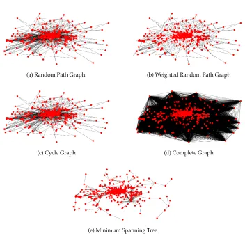
Spatial graph construction
(a) Random Path Graph. (b) Weighted Random Path Graph
(c) Cycle Graph (d) Complete Graph
(e) Minimum Spanning Tree
Figure 3: Different Spatial graph structures
We tested a variety of graphs that were constructed based on different principles, in-cluding:
• Random Path Graph: A path graph is a graph that can be drawn so that all of its vertices and edges lie on a single straight line [27]. We randomly assign tweets in a line so that they are linked to each other one by one as shown in Figure 3(a). If two nodes are connected to each otherAij= 1in its adjacency matrix, otherwiseAij = 0.
• Weighted Random Path Graph:Same structure as path graph shown in Figure 3(b), however, the weights for edges are defined by spatial interaction as:
Aij = 1/(1 +distance) (6)
• Weighted Random Circle Graph: Same structure as cycle graph, however, the weights for edges are defined by spatial interaction.
• Complete Graph: A complete graph is a graph in which each pair of graph vertices is connected by an edge shown in Figure 3(c).
• Weighted Complete Graph: Same structure as complete graph, but the weights for edges are defined by spatial interaction.
• Minimum Spanning Tree:We first generate a series of graphs based on spatial adja-cency using distances ranging from 2 kilometers to 15 kilometers. We then perform minimum spanning tree for each one of those graphs to further minimise the number of connections. In Figure 3 (e) is an example of minimum spanning tree calculated starting from the 9 kilometers spatial adjacency. If two nodes are connected to each otherAij= 1in its adjacency matrix, otherwiseAij = 0.
• Weighted Minimum Spanning Tree:Same structure as minimum spanning tree, but the weights for edges are defined by spatial interaction.
5.4
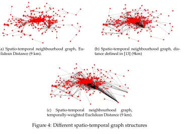
Spatio-Temporal graph
The temporal component of social media post [61] is a key aspect to take into account to move beyond the simple geotag [17]. The temporal evolution of social media trend has clear links to emerging events in the physical world [55], which leave “data shadows” be-hind them [51]. Spatio-temporal analysis has been widely adopted in the study of digital geographies [15,24,36], to identify sociospatial patterns of online events [18,41], or to mon-itor and surveillance nature disasters [43, 56]. To explore the usefulness of the temporal component of social media posts in better understanding its relationship with the assigned labels, we tested two graphs based on two different spatio-temporal distances.
• Spatio-temporal neighbourhood, Euclidean Distance: To be consistent with spatial distance, we transform the time series information equivalent to the spatial distance, and we define such process astemporal-spatial distance transformation. We will show our experiments on different setups of transformations in section 6. We define the first spatio-temporal distance as:
ST Dist= q
easting2
dist+northing2dist+time_series2dist (7)
where distance is calculated using the British National Grid3. An example of the constructed graph using Eculidean distance is shown in Figure 4(a).
• Spatio-temporal neighbourhood, temporally-weighted Euclidean Distance:Chang et al. [13] defines a spatio-temporal similarity measure to compute spatio-temporal relevance between two trajectories of moving objects on road networks, which is known as spatio-temporal distance:
ST Dist= (SD+δ∗T D)/2 (8)
whereδ is the spatio-temporal weight; SDand TDdenote for spatial distance and temporal distance respectively. An example of using such distance can be seen in Figure 4(b). As each entity in our dataset represents a point in the space-time con-tinuum, rather than a trajectory, we propose the following definition of the distance
(a) Spatio-temporal neighbourhood graph, Eu-clidean Distance (9 km).
(b) Spatio-temporal neighbourhood graph, dis-tance defined in [13] (9km)
(c) Spatio-temporal neighbourhood graph, temporally-weighted Euclidean Distance (9 km).
Figure 4: Different spatio-temporal graph structures
between two points into:
ST Dist=pSD2/2 + (δ∗T D)2/2 (9)
where we keepδ as 20 same in [13], SDis defined as peasting2
dist+northing
2
dist. It is an variation of the Euclidean distance, but taking into account of an additional spatial weight defined in formula (8) to define the impact of the temporal distance. Thus, we define such approach asTemporal weighted Euclidean Distance. An example of the constructed graph using temporal weighted Euclidean distance is shown in Figure 4(c).
• Spatio-temporal neighbourhood, distance and temporally weighted Graph:Given the best results reported in section 6 is achieved by using graph defined by Equation 9, I define this graph same structure as the temporally weighted Euclidean Distance model, but the weights for edges are defined by spatial-temporal interaction as:
Aij = 1/(1 +distanceST) (10)
wheredistanceST is the distance calculated by Equation 9.
5.5
Baseline methods
• SVM: We adopt a traditional machine learning approach Support Vector Machine (SVM) [16] on the extracted representations from multi-modal autoencoder to classify tweets.
• Dense Neural Network (DNN): We adopt a 3-layer dense neural network (DNN) on the extracted representations from multi-modal autoencoder to classify tweets.
• Visual-textual Fused CNN (VTCNN): Inspired by Huang et al. [31], we design an end-to-end deep learning framework using two stacked CNN to extract representa-tions from images and text simultaneously, and concatenate them in the middle layer of the framework to classify tweets.
• Doc2Vec + Label Propagation: We use Doc2Vec [35] to extract text representation and a traditional semi-supervised machine learning approach Label Propagation (LP) [64] to classify tweets.
• Doc2Vec + GCN (Spatial Graph): We use Doc2Vec to extract text representation and GCN on a spatially constructed graph to classify tweets.
• LSTM autoencoder + GCN (Spatial Graph): We use a LSTM autoencoder to extract text representation and GCN on a spatially constructed graph to classify tweets.
• CNN autoencoder + Label Propagation: We use a CNN autoencoder [42] which is the same structure as we adopted in the multi-modal autoencoder to extract image representation, and use LP approach to classify tweets.
• CNN autoencoder + GCN (Spatial Graph): We use the CNN autoencoder to extract image representation, and GCN on a spatially constructed graph to classify tweets.
With the exclusion of the baseline VTCNN, which is an end-to-end training framework, representation extraction (from images, text or both) and classification are two separated steps. SVM, DNN and VTCNN are baselines designed for comparisons on combined rep-resentations from multimedia content (images and text). The other five baselines are de-signed to use only one channel (images or text).
5.6
Model training
The text content of each tweet was pre-processed using tokenization, stop words removal and case folding. The resulting text was then vectorized using Word2Vec, a publically available word embeddings model trained with a 400 million Twitter dataset4.
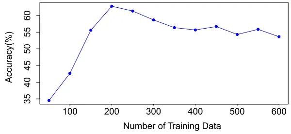
The image content of each tweet was converted to grey scale and re-size them into 158*158 uniform size images. After the extraction of the encoded features using the en-coder component of the autoenen-coder has been completed, we randomly selected certain amount of tweets (as discussed below) from the dataset as training data for the GCN. The number of tweets in each category in the dataset is unbalanced, we ensured that at least four tweets from each categories were selected in the training sample. For the same reason, we evaluated our model based on both the classification accuracy and F1 score.
We train a two-layer GCN model with 0.5 dropout rate for both layers,L2 regulariza-tion factor for the first GCN layer and 8 as the number of hidden units. We train the GCN model for a maximum of 3000 epochs (training iterations) using Adam [33] with a learning rate of 0.01, and early stopping with a window size of 300, that is the model stop training if the validation loss does not decrease for 300 consecutive epochs. Trainable weights ini-tialization and feature vectors normalization remain the same as in [34]. Our framework is
designed in Keras5with Tensorflow6as backend, and the training producer was performed
using Nivida GPU Geforce GTX 10807.
100 200 300 400 500 600
35
40
45
50
55
60
Number of Training Data
Accu
racy(%)
Figure 5: Variation of accuracy based on the number of training data.
Figure 5 illustrates the curve for the training accuracy by randomly sampling the num-ber of tweets as training data various from 50 to 600, increment by 50. The test is performed using the Random Path Graph structure, and it shows that the best number of samples is around 200. Once the size over 200, there is a slight drop on the performance of the GCN, and the accuracy tends to be stable. The reason behind why the performance drops after the number of training data more than 200 is that the training data are becoming too un-balanced that the model could properly handle, whereas when the number of tweets fewer than 200, model is struggling to perform desired classifications without sufficient training samples. The result demonstrates that our framework can achieve a reasonably good result with only partially labeled data.
6
Results
6.1
Spatial graph
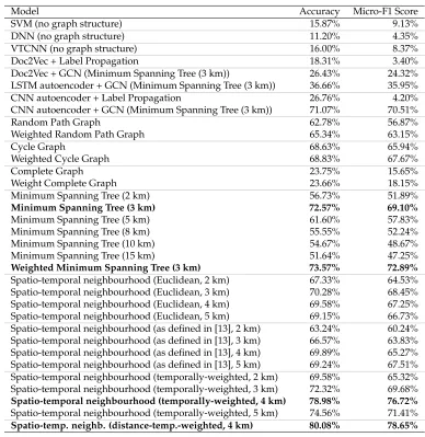
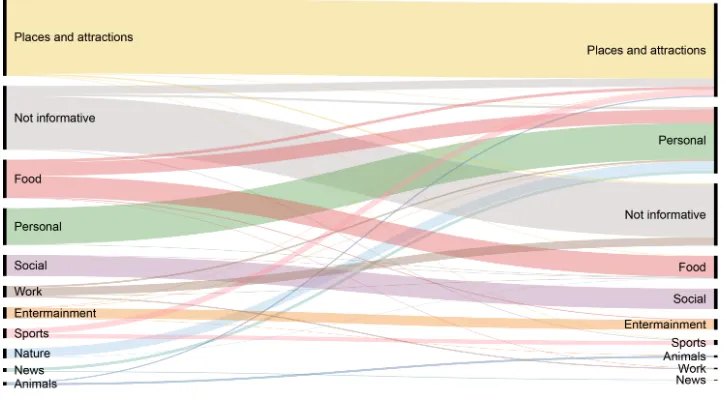
As summarized in Table 1, the results reveal that our best GCN approach successfully cat-egorize each tweet into its corresponding category based on partially labeled data with an accuracy of72.57%. Figure 6 shows how the manually assigned labels compare to the model output, and it illustrates how most of the errors are due to someFoodand most of
Naturetweets being labelled asPersonalby the model, manySportstweets being labelled as
Places and attractions, and mostWorktweets being labelled asNot informative. Errors do not seem to display any specific spatial pattern.
Those result is achieved on a training sample of 200 randomly selected tweets and de-spite a fairly imbalanced and noisy dataset. The GCN seem to perform better on a sim-ple graph structure, as the best results are obtained with a graph structure constructed by
5https://keras.io/
6https://www.tensorflow.org/
Model Accuracy Micro-F1 Score
SVM (no graph structure) 15.87% 9.13%
DNN (no graph structure) 11.20% 4.35%
VTCNN (no graph structure) 16.00% 8.37%
Doc2Vec + Label Propagation 18.31% 3.40%
Doc2Vec + GCN (Minimum Spanning Tree (3 km)) 26.43% 24.32% LSTM autoencoder + GCN (Minimum Spanning Tree (3 km)) 36.66% 35.95% CNN autoencoder + Label Propagation 26.76% 4.20% CNN autoencoder + GCN (Minimum Spanning Tree (3 km)) 71.07% 70.51%
Random Path Graph 62.78% 56.87%
Weighted Random Path Graph 65.34% 63.15%
Cycle Graph 68.63% 65.94%
Weighted Cycle Graph 68.83% 67.67%
Complete Graph 23.75% 15.65%
Weight Complete Graph 23.66% 18.15%
Minimum Spanning Tree (2 km) 56.73% 51.89%
Minimum Spanning Tree (3 km) 72.57% 69.10%
Minimum Spanning Tree (5 km) 61.60% 57.83%
Minimum Spanning Tree (8 km) 55.55% 52.24%
Minimum Spanning Tree (10 km) 54.67% 48.67%
Minimum Spanning Tree (15 km) 51.64% 47.25%
Weighted Minimum Spanning Tree (3 km) 73.57% 72.89%
Spatio-temporal neighbourhood (Euclidean, 2 km) 67.33% 64.53% Spatio-temporal neighbourhood (Euclidean, 3 km) 70.28% 68.45% Spatio-temporal neighbourhood (Euclidean, 4 km) 69.58% 67.25% Spatio-temporal neighbourhood (Euclidean, 5 km) 69.15% 66.73% Spatio-temporal neighbourhood (as defined in [13], 2 km) 63.24% 60.24% Spatio-temporal neighbourhood (as defined in [13], 3 km) 66.57% 63.83% Spatio-temporal neighbourhood (as defined in [13], 4 km) 69.89% 65.27% Spatio-temporal neighbourhood (as defined in [13], 5 km) 69.24% 67.51% Spatio-temporal neighbourhood (temporally-weighted, 2 km) 69.58% 65.32% Spatio-temporal neighbourhood (temporally-weighted, 3 km) 72.32% 69.68%
Spatio-temporal neighbourhood (temporally-weighted, 4 km) 78.98% 76.72%
Spatio-temporal neighbourhood (temporally-weighted, 5 km) 74.56% 71.41%
Spatio-temp. neighb. (distance-temp.-weighted, 4 km) 80.08% 78.65%
Table 1: Comparisons of different graph structures. (Best results achieved.)
creating weighted minimum spanning tree using a 3 kilometers range, whereas the classi-fication accuracy and F1 score on the two complete graphs are much lower compared to the other spatial graph structures. Clearly, choosing a suitable distance range for creating graph structure will be essential in further developing our framework. The results shows that the finding a geographic graph that has an appropriate density of connections within a reasonable distance range can significantly improve the performance of our graph-based semi-supervised framework.
re-Figure 6: Comparing manually assigned labels and the output from the model based on a Minimum Spanning Tree (3 km).
sults shows a even better accuracy of73.57%, and it illustrates that knowing local context (i.e., tweets posted nearby) can help our framework to better understand content.
We also compare our semi-supervised framework with a traditional supervised learn-ing method SVM, that performed the classification purely based on the exacted features from the stacked multi-modal autoencoder and their corresponding categories, with no geographical knowledge. As discussed above, the labels used in the case study are not geographical per-se, but only based on the textual and image content, that is the same in-formation provided to the SVM. As shown in Table 1, our GCN framework outperforms this traditional supervised machine learning method. Moreover, as evident by further ex-periments, our proposed framework outperforms the two deep learning methods DNN and VTCNN. It is important to highlight that these two frameworks were originally de-signed for supervised learning tasks with large and well-defined training data. In the con-text of our task, those two frameworks are inevitably overfitted during training phrase with only 200 training data points, which is considered as a relatively small and noisy sample. However, the problem of insufficient training samples is never an issue for GCN framework. These findings are particularly interesting from a geographic perspective. The GCN approaches are clearly superior to the traditional supervised learning model, and the Minimum Spanning Tree approach, which encodes the geography of the tweets, is able to outperform the other approaches, which use random or complete graphs. As labels used are not geographical per-se and have not been assigned based on the tweet’s location, this seem to indicate that the geographies of tweets can provide a valuable insight into their content.
rather than using combined representations for the classification. As GCN with spatial graph constructed using minimum spanning tree with 3 kilometers as radius achieves rea-sonably well classification, we implement the same settings for GCN models in the baseline experiments. The result shows that the GCN model outperforms the traditional machine learning semi-supervised approach Label Propagation. Also, the classification solely re-lying on text content proves to be unreliable with a comparably low accuracy. Further-more, although the classification on image content achieves worse results compared with multimedia content, it produces a competitive classification output with a relatively high accuracy and F1 score. This is particularly interesting from social science perspective, as it proves the evidence that visual content offers richer complementary information than what the accompanying text reveals [10], and human judgment is dominated by the image content of tweets at the labeling stage.
6.2
Spatio-Temporal graph
As mentioned in Section 5.4, to be consistent with spatial distance, we transform the time series information equivalent to the spatial distance. In Table 1, we summarise the results of experiments on spatio-temporal graphs using 10meter=12hours(see next paragraph for further discussion). The topological structure using Minimum Spanning Tree based on temporal weighted Euclidean distance with radius as 4 kilometers achieves the best results for both accuracy (78.98%) and F1 score (76.72%). A further performance improvement is obtained when applying the weighted minimum spanning tree using same distance radius (80.08%accuracy and78.65% F1 score). The performance is superior compared with the results achieved by spatial graphs discussed above. The findings also illustrate that despite the variation of the graphs constructed using different types of spatio-temporal distance and distance radius, the results achieved prove to be rather stable with higher accuracy and F1 score comparing with spatial graphs. These findings are interesting from spatio-temporal analysis perspective, as they illustrate that adding spatio-temporal component of tweets can help the GCN model to produce a better semantic categorization on their multimedia contents.
We also design further experiments using different temporal-spatial distance transfor-mations on the graphs, and explore their impacts on classification accuracy. As shown in Table 1, the best results for graphs constructed using Spatio-Temporal Euclidean Distance and Temporal Weighted Euclidean Distance are achieved with radius equal to 3 and 4 kilo-meters. As such, we use 3 and 4 kilometers as default radius to construct graphs respec-tively for these two approaches. Table 2 shows the results obtained on different temporal-spatial distance transformations including 1meter = 12hours, 10 meter =6 hours, 10
meter=8 hours, 10meter =12hoursand 10 meter =24hours. These test allowed us to test different temporal “localities” and how they compare against spatial “localities” in capturing events and spatio-temporal patterns. The results indicate that 10 meter =12
hoursperforms best in the context of our dataset.
dis-Transformations Spatio-temporal Euclidean Distance Temporal Weighted Euclidean Distance
1m = 12hr 60.53% 65.56%
10m = 6 hr 65.47% 72.08%
10m = 8 hr 68.23% 75.82%
10m = 12 hr 70.28% 80.08%
10m = 24 hr 68.85% 77.07%
Table 2: Comparisons between different temporal-spatial distance transformations. (Best results achieved.)
tance in deep learning approach to achieve semantic understandings on the content anal-ysis. How to best model spatio-temporal distance in this context is an interesting research area that we hope to explore further in our future work.
6.3
Framework Robustness
As mentioned in Section 4, the dataset used for the experiments presented in this paper is noisier and more imbalanced than classic benchmarks used in traditional classification tasks. It is therefore important that we explore the effects of such imbalances on the classi-fication task, and evaluate the robustness of our framework against variations in training data.
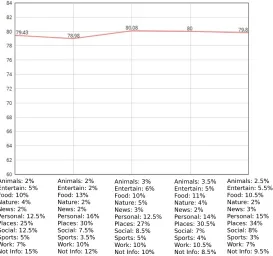
Figure 8: Results of the prediction test on a further unlabeled sample.
Therefore, we design an additional experiment using five different samples from our datasets. Each sample has at least four tweets for each category, but the proportion of tweets in the different categories is slightly adjusted. The experiment is conducted using the best performing approach in Table 1, that is a weighted graph constructed using the temporal weighted Euclidean distance with weighted minimum spanning tree (4 km).
The results are shown in Figure 7. Although model performance is slightly affected by the variation in the sample, the classification results are fairly consistent and stable. The re-sults illustrate the robustness of our proposed framework on heavily imbalanced datasets such as “live” social media streams, and thus its relevance for applications in digital ge-ographies.
6.4
Results showcase
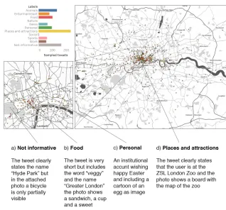
loca-tion in a park and a text that indicates being at an attracloca-tion with the image of a bicycle. At the same time, the remaining three tweets indicated in Figure 8 seem to have been assigned a fairly accurate label among those we defined for our case study, and considering that the aim of the tool is to allow users to define their own categories.
7
Discussion
In the sections above, we introduced a semi-supervised learning framework based on ge-ographic adjacency networks to categorise social media posts based on their textual and visual content, as well as spatial and temporal aspects. The results demonstrate that taking into account the geography of each post is crucial to achieve a semantic understanding of the (non-geographic) content and enable classification. In particular, while the labels used in the experiment were not assigned based on the location of social media posts, spatially-enabled classifiers performed better than a-spatial ones. The temporal component was also established as a key aspect in encapsulating the concept of place, and taking into account spatio-temporal relationships between social media post led to better classification. The results show that our framework can produce good classification results with partially la-belled data, even on noisy and imbalanced data such as the one used for the case study presented above. Although we used Twitter as our case study, our framework has the flex-ibility to be extended to any other social media platform providing location-based services. As such, our approach has the potential to be developed into a flexible tool for the study of digital geographies.
The majority of quantitative research on social media analysis in geography focuses on the text, whereas qualitative research maintains the importance of visual content [6]. As such, we based our work on the assumption that including the visual component of a post provides key information in understanding its content. To test that assumption we designed a set of experiments to compare the classification resulting from including both text and images, only text and only images, using our GCN model, as well as the semi-supervised approach Label Propagation [64] as our baseline. The outcomes show that the best results are provided by GCN, which takes into account the geographies of social me-dia content (more on this below), as well as text and image. That indicates that including both the textual and media component improves the classification results compared to tra-ditional text-based social media analysis, confirming our assumption above. These results are particularly important in a time where visual content such as images have become an integral and growing part of social media communication, as users shift from text-based posts to multimedia content [57]. By taking advantage of recent developments in deep learning technologies, our paper is a first step towards bridging the gap between text-based quantitative analysis and visual methodologies in digital geographies.
ran-dom or complete graph structures. The performance of our model is clearly superior to the traditional machine learning approach SVM [16], which does not take into account spatial graph structures, and classifies tweets based solely on the extracted feature representations. The comparison with the results obtained by two simpler, a-spatial deep learning frame-works (i.e., DNN and VTCNN) demonstrate that a deep neural network which takes into account the geographies of social media post provides not only better classification results compared to traditional machine learning methods, but also better results compared to state-of-art deep learning approaches. Furthermore, the outcomes obtained by using differ-ent spatial graphs demonstrate that selecting an appropriate spatial (topological) structure can significantly improve the classification results.
The results ultimately highlight the importance of understanding social media content geographically. The geotag specifying the location in space of a post is not merely a point, but it is an integral part of the augmentations that bring the place into being [25]. As such, taking into account the spatial relations between posts via the convolution of content through the spatial graphs allows us to go beyond the geotag [17], and provides the GCN with key contextual information, that is crucial in the semantic understanding of social media content and thus the digital representations of the city [8]
However, places do not merely exist in space, but they are “specific time-space con-figurations made up of the intersection of many encounters between ‘actants’ (people and things)” [3]. In fact, our experiments indicate that the semantic categorisation of social media posts benefits significantly from including not only the spatial but also the temporal aspects of social media content. We experimented with graphs based on spatio-temporal distance which take the temporal element of tweets into account during the construction of graph. We proposed two distance calculation approaches, one based on a spatio-temporal Euclidean distance and one based on a temporal weighted Euclidean distance. The former simply considers the temporal element as a third, separate dimension, whereas the latter uses a mathematical weight to equate space and time, to control the impact of time on dis-tance. These versions of the GCN thus take into account not merely the spatial neighbours of a tweet to understand the local context, but its spatio-temporal neighbours. The results show that taking into account the temporal component improves the quality of the cate-gorisation and the stability of the model. The GCN model on the graph constructed using temporal weighted Euclidean distance also achieves the overall best results, which does not only illustrate the effectiveness of our distance calculation approach but also indicates that a social media analysis requires sophisticated modelling of the temporal element. The GCN seems to successfully capture the in-depth connections between similar events that might be spatially distant from each other but temporally close, and vice versa.
As such, a GCN on a well-defined spatio-temporal graph achieves better results through a deeper understanding of places as “time-space configurations” [3] and social media posts as “intersection of many encounters between ‘actants’" [3], thus contextualising each post within its spatio-temporal neighbours. To the best of our knowledge, this is the first paper to embed a spatio-temporal distance into a deep learning approach to achieve semantic understandings of social media content. While our approach in this paper has achieved reasonable performance, we suggest that further research is necessary with regard to this aspect.
ro-bust and produces stable, consistent classifications. As such, we argue that our proposed framework has the potential to be developed into a powerful tool for analysis of noisy and imbalanced social media datasets in digital geographies.
8
Conclusions and Future Work
In this paper, we presented a novel approach to the exploratory analysis of geolocated social media content capable of classifying posts based not only on their textual content but also taking into account their visual content, and embedding the concept of place through spatio-temporal graph convolutional networks, thus breaking new ground in the use of deep learning in GIScience. Furthermore, our experiments show that our framework can also benefit research in digital geographies [6] in the analysis of large volumes of data, where a mixed-method approach combining quantitative and qualitative analysis might be necessary.
We outlined a stacked multi-modal autoencoder able to extract combined representa-tions from multi-media content of social media posts, and a graph convolutional network with encoded geographical information developed to classify social media posts based on the user activities they represent and the place where they are posted. The outcomes in-dicate that our framework can produce good classification results with partially labelled data, even if the dataset is heavily noisy and imbalanced. Our experiments also demon-strate that spatio-temporal graph convolutional networks are an effective way to encapsu-late and understand social media posts as “augmentations” [25] of places as “time-space configurations” [3] and thus enable a better semantic characterization of content. As such, our approach is a first step towards bridging the gap between quantitative textual process-ing and visual content analysis in digital geographies, illustratprocess-ing how visual content is an indispensable part of social media analysis, and it has the potential to be developed into a flexible tool for the study of digital geographies.
Our future work will focus on testing the scalability of our framework with a bigger and probably much noisy dataset. As discussed above, categories can have fuzzy boundaries, and even manual labelling can be a difficult and very subjective task. We are experimenting a fuzzy logic classification, where multiple labels (or “codes”) can be attached to each tweet. This approach would be well suited to case studies such as the one presented above in the field of digital geographies, where frequently more than one label can be attached to a single piece of text or image during qualitative content analysis. Moreover, as the feature extraction and semi-supervised training are separated in two subsequent stages, we are working towards combining them into an end-to-end training framework. We are also interested in better understanding the association between place, user activity types and social media posts, and how such connections can further inform our understandings of online place representation.
References
[2] ABROL, S., KHAN, L., AND THURAISINGHAM, B. Tweecalization: Efficient and in-telligent location mining in twitter using semi-supervised learning. InInternational Conference on Collaborative Computing: Networking(2012).
[3] AGNEW, J. Space and place. InThe SAGE handbook of geographical knowledge, J. Agnew and D. N. Livingstone, Eds. Sage London, 2011, ch. 23, pp. 316–330.
[4] ANDERSON, T. An introduction to multivariate statistical analysis.[una introducción al análisis estadístico multivariado].
[5] ANDREW, G., ARORA, R., BILMES, J., ANDLIVESCU, K. Deep canonical correlation analysis. InInternational conference on machine learning(2013), pp. 1247–1255.
[6] ASH, J., KITCHIN, R., AND LESZCZYNSKI, A. Digital turn, digital geographies?
Progress in Human Geography 42, 1 (2018), 25–43.
[7] AWCOCK, H. Contesting the Capital: Space, Place, and Protest in London, 1780-2010. PhD thesis, Royal Holloway, University of London, 2018.
[8] BALLATORE, A.,ANDDESABBATA, S. Los angeles as a digital place: The geographies of user-generated content. Transactions in GIS n/a, n/a. 10.1111/tgis.12600.
[9] BALLATORE, A., AND DE SABBATA, S. Charting the geographies of crowdsourced information in greater london. InGeospatial Technologies for All(Cham, 2018), A. Man-sourian, P. Pilesjö, L. Harrie, and R. van Lammeren, Eds., Springer International Pub-lishing, pp. 149–168.
[10] BORTH, D., CHEN, T., JI, R.,ANDCHANG, S.-F. Sentibank: large-scale ontology and classifiers for detecting sentiment and emotions in visual content. InProceedings of the 21st ACM international conference on Multimedia(2013), ACM, pp. 459–460.
[11] CAI, G.,ANDXIA, B. Convolutional neural networks for multimedia sentiment anal-ysis. InNatural Language Processing and Chinese Computing. Springer, 2015, pp. 159–167.
[12] CHANDAR, S., KHAPRA, M. M., LAROCHELLE, H., ANDRAVINDRAN, B. Correla-tional neural networks.Neural Computation 28, 2 (2016), 257.
[13] CHANG, J.-W., BISTA, R., KIM, Y.-C., AND KIM, Y.-K. Spatio-temporal similarity measure algorithm for moving objects on spatial networks. InInternational Conference on Computational Science and Its Applications(2007), Springer, pp. 1165–1178.
[14] CHEN, M., ZHANG, L.-L., YU, X.,ANDLIU, Y. Weighted co-training for cross-domain image sentiment classification. Journal of Computer Science and Technology 32, 4 (2017), 714–725.
[15] CHENG, T., AND WICKS, T. Event detection using twitter: a spatio-temporal ap-proach. PloS one 9, 6 (2014), e97807.
[17] CRAMPTON, J. W., GRAHAM, M., POORTHUIS, A., SHELTON, T., STEPHENS, M., WILSON, M. W., ANDZOOK, M. Beyond the geotag: situating ‘big data’ and lever-aging the potential of the geoweb.Cartography and Geographic Information Science 40, 2 (2013), 130–139. 10.1080/15230406.2013.777137.
[18] CRAMPTON, J. W., GRAHAM, M., POORTHUIS, A., SHELTON, T., STEPHENS, M., WILSON, M. W., ANDZOOK, M. Beyond the geotag: situating ‘big data’and lever-aging the potential of the geoweb. Cartography and geographic information science 40, 2 (2013), 130–139.
[19] DAN, X., PENG, C., ZHU, W., AND YANG, S. Find you from your friends: Graph-based residence location prediction for users in social media. InIEEE International Conference on Multimedia Expo(2014).
[20] FELT, M. Social media and the social sciences: How researchers employ big data analytics.Big Data & Society 3, 1 (2016), 2053951716645828. 10.1177/2053951716645828.
[21] FRIAS-MARTINEZ, V.,AND FRIAS-MARTINEZ, E. Spectral clustering for sensing ur-ban land use using twitter activity. Engineering Applications of Artificial Intelligence 35
(2014), 237–245.
[22] GAJARLA, V.,ANDGUPTA, A. Emotion detection and sentiment analysis of images.
Georgia Institute of Technology(2015).
[23] GAO, Y., ZHAO, S., YANG, Y.,ANDCHUA, T.-S. Multimedia social event detection in microblog. InInternational Conference on Multimedia Modeling(2015), Springer, pp. 269– 281.
[24] GOMIDE, J., VELOSO, A., MEIRAJR, W., ALMEIDA, V., BENEVENUTO, F., FERRAZ, F., ANDTEIXEIRA, M. Dengue surveillance based on a computational model of spatio-temporal locality of twitter. InProceedings of the 3rd international web science conference
(2011), ACM, p. 3.
[25] GRAHAM, M., DE SABBATA, S.,ANDZOOK, M. A. Towards a study of information geographies: (im)mutable augmentations and a mapping of the geographies of infor-mation.Geo: Geography and Environment 2, 1 (2015), 88–105. 10.1002/geo2.8.
[26] GRAHAM, M., ZOOK, M., AND BOULTON, A. Augmented reality in urban places: contested content and the duplicity of code.Transactions of the Institute of British Geog-raphers 38, 3 (2013), 464–479. 10.1111/j.1475-5661.2012.00539.x.
[27] GROSS, J. L.,ANDYELLEN, J.Graph theory and its applications /. 1999.
[28] HOLLENSTEIN, L.,ANDPURVES, R. Exploring place through user-generated content: Using flickr tags to describe city cores. Journal of Spatial Information Science 2010, 1 (2010), 21–48.
[30] HUANG, P.-Y., LIANG, J., LAMARE, J.-B., AND HAUPTMANN, A. G. Multimodal filtering of social media for temporal monitoring and event analysis. InProceedings of the 2018 ACM on International Conference on Multimedia Retrieval(2018), ACM, pp. 450– 457.
[31] HUANG, X., WANG, C., LI, Z., ANDNING, H. A visual–textual fused approach to automated tagging of flood-related tweets during a flood event. International Journal of Digital Earth(2018), 1–17.
[32] IFRIM, G., SHI, B., AND BRIGADIR, I. Event detection in twitter using aggressive filtering and hierarchical tweet clustering. InSNOW-DC@ WWW(2014), pp. 33–40.
[33] KINGMA, D. P., AND BA, J. Adam: A method for stochastic optimization. arXiv preprint arXiv:1412.6980(2014).
[34] KIPF, T. N., ANDWELLING, M. Semi-supervised classification with graph convolu-tional networks.
[35] LE, Q., ANDMIKOLOV, T. Distributed representations of sentences and documents. InInternational conference on machine learning(2014), pp. 1188–1196.
[36] LEE, C.-H., YANG, H.-C., CHIEN, T.-F.,ANDWEN, W.-S. A novel approach for event detection by mining spatio-temporal information on microblogs. In2011 International Conference on Advances in Social Networks Analysis and Mining(2011), IEEE, pp. 254–259.
[37] LEE, R., WAKAMIYA, S.,ANDSUMIYA, K. Discovery of unusual regional social activ-ities using geo-tagged microblogs.World Wide Web 14, 4 (2011), 321–349.
[38] LIU, P., AND DE SABBATA, S. Learning digital geographies through a graph-based semi-supervised approach. In the 15th International Conference on GeoComputation
(Queenstown, New Zealanda, 2019).
[39] LIU, P., AND DE SABBATA, S. Learning digital geographies through a multi-modal autoencoder. InGISRUK 2019, the 27th annual GIScience Research UK conference (New-castle, UK, 2019).
[40] LONGLEY, P. A.,ANDADNAN, M. Geo-temporal twitter demographics. International Journal of Geographical Information Science 30, 2 (2016), 369–389.
[41] LUO, F., CAO, G., MULLIGAN, K., AND LI, X. Explore spatiotemporal and demo-graphic characteristics of human mobility via twitter: A case study of chicago.Applied Geography 70(2016), 11–25.
[42] MAO, X. J., SHEN, C.,ANDYANG, Y. B. Image restoration using convolutional auto-encoders with symmetric skip connections.
[43] MARTÍN, Y., LI, Z., AND CUTTER, S. L. Leveraging twitter to gauge evacuation compliance: Spatiotemporal analysis of hurricane matthew. PLoS one 12, 7 (2017), e0181701.
[45] MILLER, H. J.,ANDGOODCHILD, M. F. Data-driven geography.GeoJournal 80, 4 (Aug 2015), 449–461. 10.1007/s10708-014-9602-6.
[46] MOUZANNAR, H., RIZK, Y.,AND AWAD, M. Damage identification in social media posts using multimodal deep learning, 2018.
[47] O’SULLIVAN, D.,ANDUNWIN, D.Geographic information analysis. John Wiley & Sons, 2014.
[48] PANTERAS, G., WISE, S., LU, X., CROITORU, A., CROOKS, A.,AND STEFANIDIS, A. Triangulating social multimedia content for event localization using flickr and twitter.
Transactions in GIS 19, 5 (2015), 694–715.
[49] RESCH, B., SUMMA, A., SAGL, G., ZEILE, P.,ANDEXNER, J. P.Urban Emotions—Geo-Semantic Emotion Extraction from Technical Sensors, Human Sensors and Crowdsourced Data. 2015.
[50] SECHELEA, A., DOHUU, T., ZIMOS, E.,ANDDELIGIANNIS, N. Twitter data cluster-ing and visualization. In2016 23rd International Conference on Telecommunications (ICT)
(2016), IEEE, pp. 1–5.
[51] SHELTON, T., POORTHUIS, A., GRAHAM, M., AND ZOOK, M. Mapping the data shadows of hurricane sandy: Uncovering the sociospatial dimensions of ‘big data’.
Geoforum 52(2014), 167 – 179. https://doi.org/10.1016/j.geoforum.2014.01.006.
[52] SOMMER, A. The utility of “big data” and social media for anticipating, preventing, and treating disease.JAMA ophthalmology 134, 9 (2016), 1030–1031.
[53] TSOU, M.-H., YANG, J.-A., LUSHER, D., HAN, S., SPITZBERG, B., GAWRON, J. M., GUPTA, D., AND AN, L. Mapping social activities and concepts with social media (twitter) and web search engines (yahoo and bing): a case study in 2012 us presidential election.Cartography and Geographic Information Science 40, 4 (2013), 337–348.
[54] WAKAMIYA, S., LEE, R.,AND SUMIYA, K. Urban area characterization based on se-mantics of crowd activities in twitter. InInternational Conference on GeoSpatial Sematics
(2011), Springer, pp. 108–123.
[55] WANG, Z., YE, X., AND TSOU, M.-H. Spatial, temporal, and content analysis of twitter for wildfire hazards.Natural Hazards 83, 1 (2016), 523–540.
[56] WANG, Z., YE, X.,ANDTSOU, M.-H. Spatial, temporal, and content analysis of twit-ter for wildfire hazards. Natural Hazards 83, 1 (Aug 2016), 523–540. 10.1007/s11069-016-2329-6.
[57] WELLER, K., BRUNS, A., BURGESS, J., MAHRT, M.,ANDPUSCHMANN, C.Twitter and society, vol. 89. Peter Lang, 2014.
[58] XIE, J., GIRSHICK, R., ANDFARHADI, A. Unsupervised deep embedding for cluster-ing analysis. InInternational conference on machine learning(2016), pp. 478–487.
[60] XU, Z., LIU, Y., ZHANG, H., LUO, X., MEI, L., AND HU, C. Building the multi-modal storytelling of urban emergency events based on crowdsensing of social media analytics. Mobile Networks and Applications 22, 2 (2017), 218–227.
[61] YANG, J.,ANDLESKOVEC, J. Patterns of temporal variation in online media. In Pro-ceedings of the fourth ACM international conference on Web search and data mining(2011), ACM, pp. 177–186.
[62] YOU, Q., LUO, J., JIN, H., AND YANG, J. Robust image sentiment analysis using progressively trained and domain transferred deep networks. InAAAI(2015), pp. 381– 388.
[63] ZAHRA, K., OSTERMANN, F. O.,ANDPURVES, R. S. Geographic variability of twitter usage characteristics during disaster events.Geo-spatial information science 20, 3 (2017), 231–240.
[64] ZHU, X., AND GHAHRAMANI, Z. Learning from labeled and unlabeled data with label propagation. Tech. rep., Citeseer, 2002.