California State University, San Bernardino California State University, San Bernardino
CSUSB ScholarWorks
CSUSB ScholarWorks
Theses Digitization Project John M. Pfau Library
1995
Describing and distinguishing knots
Describing and distinguishing knots
Lisa A. Padgett
Follow this and additional works at: https://scholarworks.lib.csusb.edu/etd-project Part of the Mathematics Commons
Recommended Citation Recommended Citation
Padgett, Lisa A., "Describing and distinguishing knots" (1995). Theses Digitization Project. 1102. https://scholarworks.lib.csusb.edu/etd-project/1102
DESCRIBING AND DISTINGUISHING KNOTS
A Project
Presented to the
Faculty of
California State University,
San Bernardino
In Partial Fulfillment
of the Requirements for the Degree Master of Arts
in
Mathematics
by
Lisa A. Padgett
DESCRIBING AND DISTINGUISHING KNOTS
A Project
Presented to the Faculty of
California State University,
San Bernardino
by
Lisa A. Padgett
June 1995
Approved by;
nt Chair
Dr. Gary Giiffing; Project Chair
Dr. J;>ef\Stern |
'( S~
ABSTRACT
the theory of knots has recently become a "hot" topic in mathematics,
although the study of knots began in the early 1900's. The most important
question when dealing with knots is whether two knots are actually equivalent,
i.e., whether one knot can be manipulated into the other knot without cutting or
splicing the knot. Different fields in mathematics are used to help us distinguish
knots, such as topolbgy and algebra, t will explain the different approaches
starting with the older methods involving groups up through the more modern
techniques; The theory of knots deals with a vast amount of mathematics, so in
some areas I will only touch on the subject and leave it for the reader to
ACKNOWLEDGEMENTS
I would like to thank my husband Terry/for all his love and support
throughout these past years while I have been working on my masters. I would
also like to thank all my professors while here at CSUSB, especially the
following who sparked my interest in several areas of mathematics: Dr. Gary Griffing. Dr. Zahid Hassan, Dr. Joel Stein, Dr. Peter Williams and Dr. Robert
ABSTRAGT . . . . . . v - Jii
ACKNOWLEDGEMENTS . . . . v > v :. iv
iNtRODUCTION . . 1 ... ^v: . 1
'QWAPTER:L;,r:
Knot Groups and Invariance . . ... . ... .
CHAPTER II
More Modern Techniques ^ .
Almost ©veryon© is familiar with knots in som© form or anoth©r. For
©xample, wh©n tying sho© lac©s, th© tr©foil knot is us©d. By connecting th© ©nds
of th© shoe laces after performing th© initial knot when tying your shoes, you
have the trefoil knot as shown below.
Knot Trefoil Knot
In mathematics, it is essential that we splice the ends together to form one continuous curve so that two knots can be compared. This leads to the following
definition; A knot is a simple closed polygonal curve in R^; A knot is considered
to be a subset of 3-dimensional space which is homeomorphic to the circle.
Recall, two topological spaces X and Y are called homeomorphic if there is a
continuous bijective mapping from X to Y whose inverse is continuous. We will
give 2-dimensiohal representations of knots as shown above. Even though
knots exist in R^, we will need to write them down so we will use 2-dimensionai
The most important question when dealing with knots is whether two knots, such as the trefoil and figure eight, are "equivalent".
Trefoil Knot
Figure-eight Knot
If we could manipulate one knot into the other by moving it around without
cutting or retying, then the two knots are said to be equivalent. Formally, knots
Ki and K2 are said to be equivalent if there exists a homeomorphism of
onto
Itself which maps K.) onto K2. If two knots are equivalent, they are said to be of
the same knot tvoe. A particular question of equivalence occurs when we have
a knot Ki and the unknot O = K2. In this case, if
is equivalent to K2, then
K., is said to be unknotted
Algebraic objects called invariants are used to determine whether two
knots are of the same knot type, i.e., are equivalent knots. The geometric
problem of manipulating one knot into another can be very difficult, so we
change it into an algebraic problem which hopefully will be easier to solve. Let
I
and K2 are equivalent knots(in the tppological sense), then their invariants 1^
and I2 must be equivalent(in the algebraic sense).
Therefore, using the cQntrapositive, if invariants li and I2 are not
equivalent, then the knots
and K2 are not equivalent. But if the invariants
are equivalent, nothing has been proven. It is only when the invariants are shown to be inequivalent that we can conclude that the knots must be
inequivalent. Thus, the use of invariants helps us only to prove two knots are
inequivalent. If the invariants of two knots
and K2 are inequivalent, then
cannot be manipulated into K2 no matter how hard we try or how clever we are. In the late twenties/early thirties, Reidemeister showed two knots and
K2 are equivalent if and only if
can be turned into K2 by a finite sequence of
"moves". These moves are called the Reidemeister moves and are shown
below. (Whsre in each diagram, only the relevant portion of the knot is shown.)
II
3 c
TA
III TV =
"' X "
X-The first invariant I began studying was a certain group associated with a
knot in R^. It can be shown that knots of the same type have isomorphic groups.
Given two knots, if one can show that their corresponding groups are not
isomorphic, then the two knots are not equivalent. Groups associated with knots
are given by presentations, i.e., a collection of generators and relations. Two
groups are said to be of the same presentation type if they have "isomorphic
presentations". (Two presentations are isomorphic if one can be obtained from
the other using a finite sequence of Tietze Transformations, examples later.)
In the theory of groups, the problem of determining whether two
presentations give isomorphic groups is, in general, unsolvable. So, since
determining whether two groups are isomorphic can sometimes be very difficult,
we must consider other invariants. One ofthese invariants is the sequence of
elementary ideals which are defined in terms of the matrices formed using the
presentation of the group. Another invariant is the sequence of Alexander knot
polynomials which can be defined in terms of the elementary ideals. Since each
new invariant is defined in terms of the previous, the new invariants will not give
us any more information than the previous ones did; however,the new invariants
may be easier to distinguish, easier to calculate, and easier to algebraically
manipulate. Later, I will show the use of each invariant and how each invariant
contains less information than the preceding one(knot polynomials containing
Knot type
I
Presentation type
■ ; i . .
Sequence of elementary ideals
i, .
Sequence of knot polynomials
After examining the invariants above, I will show that these are not "strong
ehough" invariants to distinguish the granny knot and square knot(shown
below). That is, each of the invariants in the list above are equivalent for both
the granny knot and square knot.
Granny Knot
Square Knot
(Remember,invariants being equivalent does not necessarily imply knots are
equivalent. Only if invariants are inequivalent can we conclude knots are
inequivalent.)
Although these knots look very similar and the invariants above are all
equivalent, we will later show it is not possible to turn one into the other no
matter what we do. We will use more modern invariants to prove that the granny
Alexander polynomial,the mpre general Jones poiynorhial, end iii sorne sense
the most general Homfly polynomial. The Homfly polynomial was so named
CHAPTER I
KNOT GROUPS
The first invariant 1 studied was the fundamental group of the complement
of a knot. To understand this invariant, we first need to understand the
fundamental group for an arbitrary topological space X. Then we will investigate
the applications of the fundamental group to knot theory. For a topological
space X, a path a is a continuous mapping a:[0, tg]- X,where tg is the
stopping time, tg ^ 0. A path a has initial point, a(0), and terminal point, a(tg),
in X. The two paths
a(t) =(i;t)
ib(t) -^1, 2t) 0 ^ t ^ 2n
are distinct even though they have the same stopping time,(2n). same initial
point,(1, 0), same terminal point,(1, 2n),and same set of image points. To be
equal paths, a and b must have the same domain of definition, i.e., terminal
points are the same,tg =^ tb and for every t in that domain, a(t)= />(t)(paths are
the same at any point in time). Consider two paths a and /> in X, where the
terminal point ofa coincides with the initial point of/), i.e., a(tg)= /)(0). The
product a• /) is
i a(t)
OstsU
The following are equivalent;
1. a • b and b • C are defined
2. a • (^ • c)is defined
3. (a'b)'C \s defined
When one of them holds,the associative jaw a * (b c) (a b) C i
A path a is called an ideality CSlh if it has a stopping time t,= 0. The path e is
identity if e
■
a = a and b-e = b. a' is the ioystsaEatilformed by
traversing a in the opposite direction. Thus, a''(t)= a(t,-1) 0 s t s A
path whose initial and terminal points coincide is called aloap- A loop's
common endpoint, p, is its basgEoint. The loop with basepoint p is referred to
as a n-hased loop. The product of any two p-based loops is again a p-based
loop. The identify path at p is a multiplicative identity. Therefore,the set of all
P-based loops in X is a semi-group with identity. By adding the notion of
equivalent paths,m can consider a new set whose elements are the equivalent
classes of paths. Thefundamental group is obtained as a combination of this
construction with the idea of a loop. Path a is said to be eguiyalsDlto path fe
(written a - ft)if and oniy if one can be continuously deformed into the other in
the topological space X without moving the endpoints. Examples of equivalent
a - b- e, since b can be shrunk to a then both a and b can be
pulled into the basepoint p.
C ~ d, since the loops in d can be rernoved.
a -i- d, Since cf cannot be pulled across the hole in the topological
// // ///
1
%
// / y //'/
/// a
/vy/.
// >0
//
V;/.
/ ••" //■ / / / z .••' .:' ; V //
v/'/cy^y-v
•>'/■■■/y//yy%y///y?%^
/ ■• / ' ' / / ^ / / / /.' / > •/ •/•• •• / / ' ■< > •'
The application of thefundamental group to knot theory changes the focus from
an arbitraiV topological space to the complementary space of a knot. The
rnmplfimfintan/ soace of a knot K,consists ofall ofthose points of
that do
not belong to K. and is denoted
- K. To explain the fundamental group of
the complement of a knot, I will use the tube model of the trefoil knot shown
below.
Let
- K be the complement of the knot and p be a fixed base point. The set
n is made up of loops in R^ - K that begin and end at p. Since O is infinitely
large, we divide n into classes of equivalent loops, a and b are equivalent
means a can be deformed into b, i.e.. a can be pulled, pushed,twisted or even
cannot come in contact with any segment of the knot. For example, in the
picture above,loop a is equivalentto loop b since a can be pulled back to b.
Also, C can be untwisted and shrunk back to the base point p(so C is equivalent
to the identity loop e). Deformationsof this type are called homotopies, and
loops such as a and b that differ only by a homotopy are said to be homotopic.
The class of loops homotopic to the loop a is written [a]. The set of loops H
can now be regarded as a collection of homotopy classes. Multiplication of
classes is defined as follows; the product[a][b] is the path that begins at p,
follows a back to p, and then follows b back to p. Multiplication of classes is an
associative operation, so([ap])[C] = [aKMc]). The class[e]acts as an
identity element,soia][e] = [e][al = [a]. Also,for every element[a] there
exists an inverse[al ^ such that[a][aj'= [a]'[a] = [e] Therefore,H
is a group.
The fundamental group of the complement of the knot K will be denoted
by n(R^ - K)and called the Imot croup of K(orjust the kDQlgrouB if K is
understood). This invariant can be used for distinguishing knots only if there is
some way to explicitly describe it. The knot group consists of a number of
equivalence classes of loops and can be calculated by constructing afinite list of
objects that will completely describe the group. This list will consist of a number
This list of generators and relations is known as a presentation of the knot
group.
Next, I will explain how we get the generators and relations for the
presentation of a knot group. I will need to explain about paths and
corresponding notation for a knot.
A knot is divided into two classes of closed, connected segmented arcs,
which are the overpasses and the underpasses. The overpasses and
underpasses alternate around the knot. The overpasses are marked below in
heavy lines, and labeled x.| , X2 , . • •
X2
Each presentation is made with respectto an orientation ofthe knot K. One of
the two directions along the knot is chosen as positive. We draw an arrow on K
to mark the positive direction. If we fix a base point p in
- K. then each loop
is defined as follows:
a* = Xj • • • X:
'■1, 'ic-'
where overpasses crossed under by a are, in order, , , Xj^, and Op == 1 or
-1 depending on whether a crosses under x, from right to left or from left to right (in other words, according as x, and the portion of the loop under X,
form a right-handed or left-handed screw). Below is an example of a loop a*
that winds under the trefoil knot:
X2 «# _ XX -U, -1
It can be shown, that the loops x, • •, X; * are the generators of the knot
group. Each loop goes under and over the overcrossing of the knot, so each loop contributes one Xj. (There are no contributions when ah overcrossing is
passed from above, only when passed from below.)
x/ = Xi
= X2
X3* = X3
X X
From now on, we will write X:'= x. and call x. /'-.x. the generators for the
knot group. Since the generators are in one-to-one correspondence with the overcrossings,from now on we will omit the diagram showing the loops that represent the generators. The relations are formed by drawing loops under and
V* =
This loop \/i that is drawn under and around one of the knots crossings can be
shrunk back to the base point p, so the loop is equivalent to the identity loop e.
[To see why the relationship among the generators at this crossing is given by
this diagram, see C. Kosniowski's"A First Course in Algebraic Topology".]
Therefore, we get the relation
X3 = 1. There are two more relations
using the trefoil knot as shown below.
V
Therefore, the presentation for the knot group of the trefoil knot is
n(R^ - K)= |Xi. X2, X3: Xi'^Xg-^XsXa = 1, Xg-^Xs'^XiXs = 1, Xi-''x3-^XiX2 =11.
It can be shown that any one of the relations for a given knot is redundant and
can be obtained using the other relations for that knot. Below I have shown that
one of the relations for the trefoil knot is redundant. (Any one of the three can
be shown to be redundant.)
(D Xi'%"^X2X3 = 1
d) X3"^X2'^XiX2 =1
(D Xi"^X3'^XiX2 = 1
Take(D and solve for X^:
X^ — X2X3X2 •
Then substitute X., = X2X3X2' into(3), so v3/ becomes
^X3^(X2X3X2 )X2 "1)
which implies equation(D x,-Vx2X3 = 1
Therefore,(D is shown to be redundant since it can be obtained using d)and
(1).[For more information on why the generators generate and where the
relations come from and why one relation is redundant, refer to C. Kosniowski s
Therefore, we obtain for the knot group of the trefoil knot K, the
presentation 'rT(R^ - K)= ,X2,X3: X3^X2^XiX2 = 1, x^ X3 X1X2- 1[ where
\/* has been dropped. By rewriting the relations, we get the presentation
n(R3.K)= |x^, X2, X3: X3= X2'X1X2, Xi = X3-^XiX21. Since X3 is expressed
in terms of x^ and X2, we can eliminate X3 by substituting X3 = X2 V1X2 into the
other relation, so n(R^ - K) = ]Xi, X2: x^ = (X2^x., ^X2)XiX2[
|Xi, X2: X^ = X2'^X|"^X2XiX2 1. By multiplying the relation through on the left by
Xi X2 , we obtain the following common presentation of the knot group of the
trefoil knot; lx,, X2; XiX2XV = X2X1X2I.: This process of substitution
and rewrite the presentation is formally known as Tietze transformations. [For
more informatioh, see''Introduction to Knot Theory''by Crowell and Fox.]
Now that we have a presentation for the trefoil knot, we can prove that it
cannot be untied, that is, the trefoil knot is not of the same knot type as the trivial
Trivial Knot
The presentation is n(R^ - K)= 1X : I. The trivial knot has only one
generator, and therefore it has no relations. Hence,the group ofthe trivial knot
type is infinite cyclic. To prove that the trefoil knot is not of the same knot type
as the trivial knot, we must show that their knot groups are not isomophic. To
prove this, I will show thatthe knot group for the trefoil knot 1X, y. xyx - yxy I
is not infinite cyclic. To do this we must consider the symmetric group S3 which
is generated by the cycles(12)and(23). S3 is not abelian since(12)(23)
(132)and(23)(12)=(123). The presentation G ofthe trefoil knot consists of
a homomorphism of thefree group F on x and y onto G whose kernel is N,the
as IX, y: xyx = yxy [. We will now show that F/N maps homomorphically
onto a nonabelian group.
Consider the map;
0: F S3
X ^(12)
y ^(13).
extended multiplicatively. The map0 is an onto group homomorphism.
Consider the commutative diagram:
w wN
> F/N
.wN 0
L S
0(W)
0(w)
Since the mapping (j) is defined on cosets, we must show well defined. If
wN = W'N,does(l)(w N) = (|)(w' N )where w and w'are related by
\/\l' = wn, ncN ? To show(|)(wN) = (t)(w' N), I first need to show
suffice to show that0 maps the generators of N to 6.
8[xyx(yxy)-^] 8(yxy)e(yxy)
8(x)8(y)8(x)[8(y)8(x)8(y)] since 8 is
homomorphism
(12)(23)(12)[(23)(12)(23)]
(13){13)-'
Therefore 8(n)= e.
Now
(|)(w' N)
(|)[(wn)N] sincew'- wn
8(wn)
definition of mapping (j)
8(w)8(n) since 8 is homomorphism
0(w) since 8(n)= e(shown above)
(j)(wN) definition of mapping.
Therefore ^N)= , so the map is well-defined. Thus, the knot group
can be mapped homomorphicaily onto a nonabelian group. So the knot group is
nonabelian (if the knot group were abelian, then its image would be abelian)and
Another example offinding a presentatiori for a knot is done below.
V. .- w
v/= zyz'^ w"^
Jf
V2^ = zy'^x'V
V3* = x'^wxz'^
v/= wy"''w"^x
w
Figure-eight Knot
A presentation for the knot group ofthe figure-eight knot K is n(R^-K)=
IX, y, z, w: z= wzy'^, y = xyz'"", z= x'^x 1 where v/ has been dropped.
Using Tietze transformatiohs we can substitute Z = X'^ wx in the other two
relations to obtain T7(R^ - K)= IX, y, w ; x'^WX = wx^wxy - ,
y = xyx'^w'^x I. The second relation now gives w = xy'^xyx"^ and by
substituting w = xy'^xyx"^ into the first relation we obtain n(R^ - K)=
Ix, y; x^^()^"''xyx'^)x = {xy'^xyx"^)x''(xy"''xyx'^)xy''' I which can be simplified to
n(R^ - K)= IX, y : y'^xy = xy"^xyx'''y'^x I . By multiplying both sides on the
of the knot group for thefigure-eight knot n(R^ - K)
|x, y: yx'Vxy'^=^ x'^yxy"^x|.
In order to prove that the figure-eight knot is distinct from the trefoil, it is
sufficient to show that their groups are not isomorphic. Unfortunately, there is no
easy way to determine whether or not two presentations have isomorphic groups. So what is needed are some easy to caclulate algebraic quantities
which when derived from isomorphic groups, remain the same. These are the
so-called group invariants. That is, since the knot group is usually too
complicated as an invariant, we must pass to one that is simpler and easier to
handle. One such invariant is the sequence of Alexander knot polynomials.
This invariant can be used to distinguish the trefoil knot and the figure-eight knot. There is an object called the Alexander matrix which is constructed using
mappings of the free group onto itself called Fox derivatives. From the
Alexander matrix we can determine the sequence of elementarv ideals which
then gives us the sequence of Alexander knot Dblvnomials. For the rest of the chapter, we will just write down the results of our calculations without leading
reader through derivations. (For details on the calculations of fox derivatives, Alexander matrices, elementary ideals, and Alexander polynomials, the reader
should consult "Introduction to Knot Theory" by Crowell and Fox.) The
sequence of Alexander knot polynomials for the trefoil knot is Ai = 1 -1 +1^ and
eight knot is Ai= - 3t + 1 and Ak - 1 for k ^ 2. Therefore,the trefoil
and figure-eight are not equivaient knots since their Alexander knot polynomials
inequivalent. In Chapter 2, I will give a detailed description of another
invariant that is easier to calculate that will also distinguish the trefoil and the
are
figure-eight.
8
"\
Figure 1
The sequence of Alexander knot polynomials for both figure 1 andfigure
2is Ai = 21^ - 5t + 2 and Ak = 1 for
2. The sequence of Alexander knot
polynomials does not distinguish these two knots. To distinguish these knots we
must use another invariant. This invariant is the sequence of elementary ideals.
The sequence of elementary idealsforfigure 1 is
=(2F - 5t + 2)and
=(1)for k ;^ 2, where(a)means the ideal generated by a in the ring
Z[t, f""]. The sequence of elementary idealsforfigure 2is =(2F - 5t + 2),
not equivalent knots sincejhelr sequence of elementary ideals are not equal. This example verifies that the elementary ideals are stronger invariants than the
polynomials.
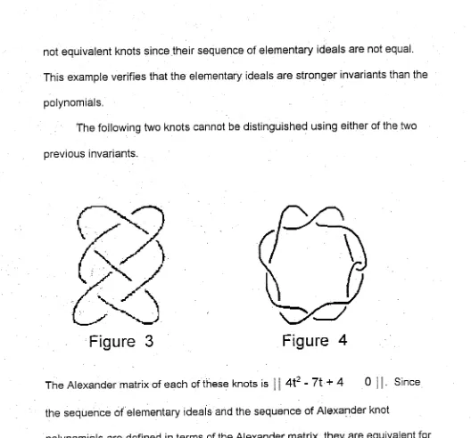
The follbwing two knots cannot be distinguished using either of the two
previous invariants.
\
Figure 3
Figure 4
The Alexander matrix of each of these knots is 1 1 4t^ - 7t + 4 0 1 1. Since
the sequence of elementary ideals and the sequence of Alexander knot
polynomials are defined in terms of the Alexander matrix, they are equivalent for
both knots. The elementary ideals and knot polynomials are not strong enough
invariants to distinguish these two knots. Although it can be shown that their
knot groups are nonisomorphic using other methods; therefore, the two knots are not equivalent. This shows the presentation type is a stronger invariant than
either the elementary ideals or knot polynomials.
they possess isomorphic groups as shown below.
Square Knot
Granny Knot
Each knot group has the presentation n(R^ - K)=|X, y, a: a xa =
xax'\ a'V^ ~ y^y ^ I • To distinguish the granny knot and square knot, we
CHAPTER II
I
In the 70's and 80's, J. H. Conway and Louis H. Kauffman each came up with a whole new approach with which to study knots. We will focus on
Kauffman's approach which uses "brackets". This new approach uses formal
symbolism and a type of arithmetic with diagrams. It also uses no fundamental
groups whatsoever. This more modern approach to knots not only is easier to
handle but can distinguish a wider variety of knots and objects to be defined
later as links.
To begin the discussion of the new approach, I mustfirst define(or in
some cases, redefine)a few terms. If we regard a knot as a single closed loop
in then a Nnk will be an object consisting of one or more such loops. As
referred to earlier, the following are the Reidemeister Moves : (Only the relevant
portion of the knot or link is shown.)
II
X
^ D C
rX
\/
andAy
\
III
\
/
if their diagrams are related by a finite sequence of Reidemeister moves. The
equivalence relation generated by moves II and III is called regular isotopy. The
equivalence relation generated by all three:moves is called ambient isotopy.
A knot or link is said to be oriented if each arc in its diagram is assigned a
direction (according to the right-handed screvv)so that at each crossing the
orientations appear either as
or
and have a corresponding sign of ±1.
Let L = {cx, P} be a link of two components ot and p.
Rpfinfi the linking number ^k(U = gk(a.|5) by the formula 5k(a,
p)-Xpeanp ^IP)' whers anp denotes the set of crossings of a with p and e(p)
denotes the sign of the crossing.
Example:
ce
,P)=%(1 +1)= 1
So the linking number of the link above is 1. Notice we only consider the
crossings of a with P,so where p crosses itself, there is no contribution to the
linking number.
Let K be any oriented link diagram. Then the writhe of K(or twist number
of KV is defined by the formula w{K)= Zp6c{K)®(P)' where c(K)denotes the set
Example:
+
w(K)= 1 + 1 + "1 + -1 + "1 = "1
Thus, the writhe of the link above Is -1. Notice all crossings were considered
when calculating the writhe.
Consider a crossing in an unoriented link diagram. Two associated
labelled diagrams can be obtained by labelling and splicing the crossing(shown
A B
B A
Type A
Type B
The regions labelled A (respectively B)are those that appear on the left
(respectively right)to ah observer walking toward the crossing along one ofthe
undercrossing segments.
By keeping track of each splice that is performed, we can reconstruct a
given knot(or link)from its descendants. A reconstruction is shown below.
A
The final descendants(that is, when all of the crossings having been
spliced) of a knot or link K are called the states of K. Each state can be used to
reconstruct K. over
these states. To do this, let 6 be a state of K and(K|6) denote the
commutative product of the labels attached to 6. Example shown below.
- A • A'A = o
Also let 1 161 1 be one less than the number of loops in 6.
=2-1 = 1
[slow we can define the bracket polynomial.(K), by the following formula.
The following is an example of the use of the bracket polynomial.
I "V. I
I I /
C®
There are four states(final descendants)for this link. The bracket polynomial is
calculated as follows;
(K) =
A^c|2-^ +ABd^-!+ ABd^-r+B2c|2-V
= A^d + AB + AB + B^dA^d + 2AB + B^d
Notice that at each node of the tree above, the bracket of the relevant
(><)= A(:rC)^B
a type B splice, so
holds(where only the relevant portion of the diagram is shown). An example of
how this can be used to compute the bracket is done below for the link L.
(l) = (noy> a/gov-b
= A (a<C£i> + b
^ B (A<Ci=0) - B<00))
= + ABd^'y + BAd^""" +
= A^d + 2AB + B^d.
Notice we got the same bracket polynomial as we did using the tree diagram.
The bracket polynomial is not an invariant as it stands. We must
investigate it under the Reidemeister moves and determine conditions on A. B,
and d for it to become an invariant. We first investigate the bracket under type II
(3C.)-^^j>J}'^{3JOj
'1 \^/y
^b(a/3cVb(
= a2/
\ + AB( O
-
B^i■:^ <r) - 02
= AB(^ O ■ )+ AB^^D c.)
/. -\
+ (a2 -H b2)(^,„—
= ABd('^)-AB(D
V(a2.B2)^^:rC)
since("~-cr') = d\'
For Xi>:> to equal ^
^ (tyP® " move), it suffices to
AB = 1 and d = -A" - A*^. Suppose A = B'" and d = -A^ - A'^ then we
have
just showed that
•^xvv = f, y
J +
/
{
i V / \( \ Using a
rr
\ Using a
l^i'^yC-S'C) * b(oI>") type
\ ^ \ //^ / move
nXxV
This shows that the bracket with B = A"\ d = -A^ - A"^ is invariant under
moves II and III. (That is, If two diagrams differ by a type II or type 111 move, their bfackets are the same.) Let's now investigate how the bracket transforms
= a(v)^Kv)
= C-a3-A-0<^)
-A'
So < n > = -A^
(-)
We will now calculate the bracket for the same diagram but with the loop
<cJ)= «(v)* Kv>
(w)- (-A^- A-^)(A-')(v--)
= A
= A
= A
= -A
«C(j)= -'-'M
Notice that if two diagrams differ by a type I move,their brackets are not the
same. Therefore, the bracket is only invariant under type II and type III moves.
To obtain an invariant of ambient isotopy (I, II and III), we must normalize
the bracket. To do this, we must take a closer look at the writhe of K, w(K).
Recall the vy(K)= EpG(p)where p runs over all crossings in K,and g(p)is the
sign of the crossing. The writhe of K is an invariant of regular isotopy (II, III) as
Type II move: (one possible orientation is shown)
= -1 +1 = 0
w
- 0
w
Since w ( >C J = '^(j!) )(independent of orientation), the
writhe is invariant under a type II move.
Tvpe III move: (again, one possible orientation is shown)
71
= 1 + -1 + 1 = 1
w
= 1 + -1 + 1 = 1
w
Since W
orientation), the writhe is invariant under a type ill move. Therefore, w(K)is an
invariant of regular isotopy. Also notice that(since writhe is sum on the
crossings).
W t ^7^ ]= 1 + w
= -1 + w
W
Now we can aefine a nnrmaliTad bracket. Jk.for °ri®rrted links K by theformula
jr =
j'r'ik)^
Iwiijshow thatthe normalized bracket of Isan
ihvariant of ambient Isotopy. Since w{K)and(K)are regular isotopy
invariants, It follows that Jk is a regular Isotopy invariant. Thus,we only need to
V
- (-A')
{15
-[ 1 + i
= (-.')
(if
.[ 1 + /
- w(^).
.
{^)
this showsJk is invariant under type I moves. Therefore, the normalized
bracket polynomialJk is an invariant of ambient isotopy.
Before 1 show the use of the normalized bracket polynomialJ[k > 'would
■ ■ f ■ ■ , ■ ■ ^
like to define the mirror image of a knot or link. The mirror image of K is
knot T and its mirror image T* are shown below. The trefoil and its mirror
image have isomorphic knot groups (left as an easy check for the reader), so
they could not be distinguished using previous methods, but using the
normalized bracket polynomial they will be shown to be distinct knots.
T /p *
Trefoil knot and its mirror image
Using the normalized bracket polynomialJk .'will show that the trefoil
knot cannot be deformed into its mirror image T*. This will show that the trefoil
i ■ ' ■ ' ' ■
Trpfnil knot T
+ A = A
-1 -1
+ A
{9
+ A = A A.
= A[A (-A^)+ A-^(-A-^)] + A-\-A-^)(-A-^)
So(T) = -A^ - A"^ + A'"^ and wC'")" ('ndependent of orientation).
Thus.Xr
= (-AT^^^HT)
= (_A3)-3(.A® - A"' + A"^)
= -A"' (-A® - A-' + A"^)
.-4 j. A-12 ,
= A^+ A"
IS
Therefore,
Mirror Image T*
= A + A
= A + A A + A
= A{-A%A^)+ A'[A(-A^)+ A"^(-A-3)]
- A-5 ■ = fij
-So <T*> = A^ - A' - A-5
and W(T*) = -3/(independent of orientation).
Thus:ir-
^
= (.A3)3(A^ - A^ - A-^)
= -A® (A^ - A^ - A'^)
= -A^ + + A^
Therefore, the normalized braeket poiynomial for the mirror image of the trefoil
kriot is Jj*- -A^® +
Since ^ , we conclude that the trefoil is
not ambient isotopic to its mirror image. That is, the trefoil knot is not
topologically equivalent to its mirror image. This is the first example of modern
In 1984, using representations of pertain algebras, V. Jones discovered a
polynomial which came to be called the Jones polynomial . The 1-variable
Jones polynomial, Vk (t). is a Laurent polynomial in the variable t (i.e.,
polynomial with integer powers of t). The polynomial satisfies:
i.
If K is ambientisotopic to K ', then V(^(t) = V|H(; i (t) .
/
■—V
iii.
- tv^ =
jt
^
^ stand for larger link diagrams that
where
differ only by the crossing shown. Jones showed that there is a unique
polynomial satisfying these identities.
I will show that the Jones polynomial is the same as the bracket
polynomial with the substitution A = t . Recall the formulas for the bracket
polynomial.
(x) = A (:r;)
By dividing the first equation by B and the second by A and solving for
we obtain the following two equations
_A
B
A-' /
-(■
\ A
By setting them equal,
B
A/
= A ■1 /B \
By regrouping like terms,
b-H
And since B - A"^ we have
A"
<
a2 - A-2 )(
;
Orientating them we obtain,
L-1 .2: - a-2
A = lA
New let a = -A^ arid multiply through by a"" where w
a
'
Va'" - A"''
df' -wFactoring outan afrom the first term and an a'"" from the second
a
a2-A-2 -w
-w
Aa<
(w*
(w -1)=(a^- A-2'
aReealllng that J[k =(-A')
■""" ( K ) allows us now to write,
Al'a"'J
Now substituting a - -A^,
The final substitution A - yields,
t'V
- t^
^
^
Therefore, with the substitution A = t into^K(A)~(-A^)
K), we notice
Jk
S3f's^'®®
defining identities for, VK(t), the Jones polynomial.
By uniqueness of VK(t). we have Jk(t
Thus,the normalized
bracket yields the 1-variable Jones polynomial.
The Jones polynomial is structurally similar to the Aleyander-Conway
pnivnorriial V.(Z)which is a polynomial in Z with integer coefficients. This
polynomial can be shown to satisfy the following properties:
i)
Vk(z)= Vki(z), if the oriented links K and K'are
ambient isotopic.
ii) vg, = 1
iii) ~ ^
Conway showed that these properties characterize this polynomial, and that this
polynomial is just a disguised and normalized form of the original Alexander
A major difference between the Jones polynomial and Conway polynomial
is that the Gonway polynomial does not differentiate mirror images. Hence, the
Conway polynomial cannot distinguish between the trefoil and its mirror image,
while the Jones polynomial can. Both the Jones and Conway-Alexander
polynomials can be generalized to what is known as the Homfly polynomial,
1PK(a,z), to be defined later. For a = t'\ Z = nIT" - sfT . Pk
specializes to the Jones polynomial, and for a = 1, Pk specializes to the
Gonway-^AIexander polynomial. Homfly Is so named after its many discoverers
(J. Hoste, A. Ocneanu, K. G. Millett, P. Freyd, W. B. R. Liekorish,0.Yetter).
The oriented inyariant PkCq,z)can be regarded as the normalization of a
regular isotopy invariant. The regular isotnpv homflv oolvnomial Hk((X, Z)
(Which we will assume exists) is defined by the following properties;
If the oriented links K and K' are regular isotopic, then
HK(a,z)= HK'(a, z).
I.
= 1
III. H ^ 1 5 = Z H
iV. H = a H
This regular isotopy Invariant can be normalized by including a to measure
the writhe in a diagram. We then have Pk(oc,z)= a HkCci,z) which is an
invariant of ambient isotopy. To prove that PK(a,z) is an invariant of ambient
isotopy. I will let P^= Pk(«.z) so Pr =
Hk(a,z). We know Pk is an
invariant of regular isotopy since w(K)and Hk(a,z) are invariants of regular
isotopy. We only need to show Pk is an invariant under type I moves. Let T.K
represent a type I move applied to K (shown below).
K :
|;;K : - y
/
!
(T)';
\
\
s.
So the question is, does P|.K - Pk '?
P,K =
a
H,K(a,z)
a-(v(K)-i)a-iHK(a,z) = a "'^^'^^a'"^a'''HK(a, z)
= a HK(a,z)
■ ■ ■ ■
eliminates a negative crossing, P.k = Pk •) W®
move
0
P^ = a°H^, since w(^)=0.
Therefore,
= 1 , sinceHgj = 1.
Since Pk is an invariant of ambient isotopy and Pi, = 1, it oniy
remainstofind ttie exchange identityfor Pk- Letw-wj
and recall that H satisfies the following identity.
Multiplying by a"'
Since da^ = 1,
-1 -W lJ n n'^ n''^ '1 — 2 Q ^ H
act 'a ^H^ - C( M a ^ ^
By rewriting,
= Z a-^ H
Therefore,
o( R ^ - a-'i R
have the hortfialized polynomial which is an invariant of ambient
We now
To show the use of the Homfly polynomial. I will calculate the Homfly
polynomial for both the trefoil and its mirror image.
Trefoil T
Recall, the exchange identity is as follows;
; hence expanding about the
- H - = ZH
negative crossing above
H - ZH
H T = H
/
Using a type II move on
the first term and the exchange identity on the second
term, we obtain;Hj - H - Z
If we apply property(iv)twice and a type II move once, we get the following:
ct - Z I - Z a-'
HT
-1
a - a
6
. Using this.Below we will show H
6' ^
we can continue and write the above as.
'°
- Za-^
= a"' - Z
= a a + a ^ +Z2a^
Therefore, since w(T) —-3,
P,(a,Z) =
Z)
= a^(2a''' -a + Z^a"'')
= 2a^ - + T}^
a -— YV-1a
(5^
Show H
,6"
6
by property (Hi).= ZH
H
0
(5'
C,_ a-1 = ZH|g I by property(iv),
■(5V
a — a"''SO H
Recall,thefollowing is the diagram for the mirror image ofthe trefoil knot T.
Mirror Image V
Again, the exchange identity is
= ZH ; hence expanding about the
positive crossing above,
H-p =
•• ^ ZH
+ ZH
the first term and the exchange identity on the second
Using a type II move on
term, we obtain;
9^
H+ Z H
Hj* -
H
If we apply property(iv)twice and a type II move once,we getthefollowing;
+ Za .
Ht* = "
0 1 _
^
so we continue:
As shown earlier H
6 "
-1
a - a
+ Za
= a + Z
'T*
= a + a - + Z^a
Therefore, since w(T)-3.
PT.(a,z) =
^ H-p(a,z)
=
a-'(2a - a*^ + z^a)
■ : =-^ 2a ^ + z^a"^
once again/1 have shown thatthe trefoil Knot and ite
this time using the Homfly polynomial/
AS mentioned earlier,the granny knot and the square knot(shown below)
nave isomorphic knot groups, and therefore could not be distinguished by using
the methods in Chapter i.
Square Knot
Granny Knot
However,the Hon^y polynomial can distinguish the granny knot and square
knot. But using the Homfly on these knots can be very tedious. To help with this
problem,one mustthink ofthese larger knots asthe"connected sum"oftwo
thatthe knots do notoverlap. Therefore,the granny knot is the oonneoted sum
of tvro trefoil knots, and the square knot is the connected sum ofa trefoil knot
and its mirror image(Shown below).
Trefoil —, Trefoi l r
P- T r e f o i 1
Square Knot
Granny Knot
it can be shown that the Homfiy ofthe connected sum oftwo knots is equal
to the product oftheir iridividuai Homfiy polynomials, i.e., Hk = Ha• Ho where
the knot K is the connected sum ofthe knotsA and B. Since the granny knot,
G, is the connected sum of two trefoils, we have
Ha =
Ht-H,.
(2a-' - a + z^a-')(2a-' - a +
= 4a-2- 2+ 2z^a-^ - 2+ a^-z^-h 2z^®-^"^
Since w(G)= -6, the normalized Homfly polynomialfor the granny knot is
Po(a,z)
a®(4a-^ - 4+
- 2z= + +z^a
=
40"- 4a® + 4zV - 2z^a® + a'+ z^ot''.
Now,since the square knot, S, is the connected sum of a trefoil and its mirror
image, we have the following;Hg - Hy * Hj.
=
(2a'^ - a + zV^)(2a - a'^ + z^a)
=
4 - 2a"^ + 2z^ - 2a^ + 1 +zV + 2z^ - z^a"^ + z^
- 5 - 2a'^ + 4z^ - 2a^ + z^a^ - z^a"^ + z"^ .
Since w(S)=0,the normalized Homfly polynomial for the square knot is
PgCa/z)= 5 - 2a-^ + 4z^ -2a^+zV-zV + z'* .
The square knot does not have the same Hornfly polynomial as the granny knot.
Therefore, they are not equivalent knots.
BIBLIOGRAPHY
E. Artin, Theory of Braids, Annals of Mathematics 48,(1947).
J. Birman, New Points of View in Knot Theory. Bulletin of the American
Mathematical Society, Volume 28, Number 2(1993), 253-287.
J. Birman, Recent Develnnments in Braid and Link Theory. The Mathematical
Intelligencer, Volume 13, Number 1 (1991), 52-60.
J. i-i Onnwav An Enumeration ofKnots and Links and some oftheir Algebraic
Properties. Computational Problems in Abstract Algebra (J. Leech, ed),
Pergamon Press, New York(1970), 329-358.
Crowell, R. H. and Fox R. H., Introduction to Knot Theory. Blaisdell Publishing
Company (1963).
L. H. Kauffman, Knots and Phvsics. \Nor\d Scientific Publishing Company Ptc.
Ltd.(1991).
L. H. Kauffman, On Knots. Princeton University Press, Princeton, New Jersey
(1987).
C. Kosniowski, A First Course in Alaetiraic Toooloav. Cambridge University
Press(1980).
C. Livingston, Knot Theory. The Mathematical Association of America,(1993).
J. R. Munkres, Tonoloav. A First Course. Prentice-Hall Inc., New Jersey(1975).
P. G. Tait, On Knots I. II. and lit. Scientific Papers of P. G. Tait, Volume 1,