An adaptive integration scheme using a mixed quadrature of three
different quadrature rules
Debasish Das,
a,∗Pritikanta Patra
aand Rajani Ballav Dash
ba,bDepartment of Mathematics, Ravenshaw University, Cuttack-753003, Odisha, India.
Abstract
In the present work,a mixed quadrature rule of precision seven is constructed blending Gauss-Legendre 2-point rule, Fejer’s first and second 3-point rules each having precision three.The error analysis of the mixed rule is incorporated.An algorithm is designed for adaptive integration scheme using the mixed quadrature rule.Through some numerical examples,the effectiveness of adopting mixed quadrature rule in place of their constituent rules in the adaptive integration scheme is discussed.
Keywords: Gauss-Legendre quadrature, Fejer’s quadrature, mixed quadrature and adaptive integration scheme
2010 MSC:65D30, 65D32. c2012 MJM. All rights reserved.
1
Introduction
In this article, we consider the following problem. Given a continuous function f(x)over a bounded interval [a,b]and a prescribed tolerancee, we seek to find an approximation Q(f)using a mixed quadrature
rule to the integral
I(f) =
Z b
a
f(x)dx (1.1)
so that
|Q(f)−I(f)| ≤e (1.2)
This can be done following adaptive integration scheme (AIS)[1] [2] [3].
Conte and Boor[3] evaluated real definite integral (1.1) in the adaptive integration scheme using Simpson’s
1
3 rule as a base rule.They fix a termination criterion for adaptive integration scheme using Simpon’s 13
two panel rule and Simpson’s 13 four panel rule (composite rule). Recently, R.B.Dash and D.Das[7] [8] [9] constructed some mixed quadrature rules and fix the termination criterion for adaptive integration using the mixed quadrature rule and evaluated successfully various real definite integrals. Mixed quadrature [5] [6] [7][8] [9] [10] [11] means a quadrature of higher precision which is formed by taking the linear/ convex combination of two or more quadrature rules of equal lower precision.
∗
Corresponding author.
The idea of mixed quadrature was first given by R.N. Das and G. Pradhan (1996) [5], who constructed a mixed quadrature rule of precision 5 blending Simpson’s 13 rule with Gauss- Legendre 2-point rule, each having precision 3. Evaluating some real definite integrals on the whole interval, they showed the superiority of the mixed quadrature rule over their constituent rules. N. Das and S.K. Pradhan(2004)[6] derived a mixed quadrature rule of precision 7 by taking a linear combination of Simpson’s 13rule,Simpson’s38rule and Gauss-Legendre 2-point rule, each having precision 3. They also showed the superiority of the mixed quadrature rule over their constituent rules by evaluating some real definite integrals in the whole interval method.
In this paper, we have constructed a mixed quadrature rule of precision 7 by mixing Gauss-Legendre 2-point rule[4] with Fejer’s first and second 3-2-point rules[2] [10] each having equal precision (i.e. precision 3) for approximating some real definite integrals in the adaptive integration scheme. The construction of mixed quadrature rule is outlined in the following section.
2
Construction of the mixed quadrature rule of precision seven
A mixed quadrature rule of precision seven is constructed by using the following three well-known quadrature rules.
(i) Gauss- Legendre 2-point rule
(ii) Fejer’s first 3-point rule
(iii) Fejer’s second 3- point rule
The Gauss-Legendre 2-point rule(RGL2(f))is
I(f) =
Z b
a
f(x)dx=
Z 1
−1
f(x)dx≈RGL2(f) = f(− 1 √
3) +f( 1 √
3) (2.3)
The Fejer’s first 3-point rule(R1F3(f))is
I(f) =
Z b
a
f(x)dx=
Z 1
−1
f(x)dx≈R1F3(f) =
1 9[4f(
−√3
2 ) +10f(0) +4f( √
3
2 )] (2.4)
The Fejer’s second 3-point rule(R2F3(f))is
I(f) =
Z b
a
f(x)dx=
Z 1
−1
f(x)dx≈R2F3(f) =
2 3[f(
−1 √
2) +f(0) +f( 1 √
2)] (2.5)
Each of these rules (2.1), (2.2) and (2.3) is of precision 3. Let EGL2(f),E1F3(f),E2F3(f)denote the errors in
approximating the integral I(f)by the rules (2.1), (2.2) and (2.3) respectively.
Then,
I(f) =R1F3(f) +E1F3(f) (2.7)
I(f) =R2F3(f) +E2F3(f) (2.8)
Assuming f(x)to be sufficiently differentiable in−1 ≤x ≤1 , and using Maclaurin’s expansion of function f(x), we can express the errors associated with the quadrature rules under reference as
EGL2(f) = 8
5!×9f(iv)(0) +7!40×27f(vi)(0) +9!16×9f(viii)(0) +...
E1F3(f) =−
1 5!×2f
(iv)(0)− 5 8!f
(vi)(0)− 17 9!×32f
(viii)(0)−...
E2F3(f) =
1
3×5!f(iv)(0) +6×57!f(vi)(0) +4×59!f(viii)(0) +...
Now multiplying the Eqs (2.4), (2.5) and (2.6) by 27, 32 and -24 respectively, then adding the results we obtain,
I(f) = 351(27RGL2(f) +32R1F3(f)−24R2F3(f)) +
1
35(27EGL2(f) +32E1F3(f)−24E2F3(f))
I(f) =RGL21F32F3(f) +EGL21F32F3(f) (2.9)
Where
RGL21F32F3(f) =
1
35(27RGL2(f) +32R1F3(f)−24R2F3(f)) (2.10)
And
EGL21F32F3(f) =
1
35(27EGL2(f) +32E1F3(f)−24E2F3(f)) (2.11)
Eq.(2.8) expresses the desired mixed quadrature rule for the approximate evaluation of I(f) and Eq (2.9) expresses the error generated in this approximation.
Hence,
EGL21F32F3(f) =
1 9!×35f
(viii)(0) +... (2.12)
As the first term ofEGL21F32F3(f)contains 8
thorder derivative of the integrand, the degree of precision of the
mixed quadrature rule is 7. It is called a mixed type rule as it is constructed from three different types of rules of equal precision.
3
Error analysis of the mixed quadrature rule
Theorem-3.1
Let f(x)be a sufficiently differentiable function in the closed interval[−1, 1]. Then the error EGL21F32F3(f)
associated with the mixed quadrature ruleRGL21F32F3(f)is given by
|EGL21F32F3(f)| ≈
1
9!×35|f(viii)(0)|
Proof The proof follows from the Eq (2.10).
Theorem 3.2
The bound for the truncation errorEGL21F32F3(f) = I(f)−RGL21F32F3(f) is given by
EGL21F32F3(f)≤
2M
175
whereM=max−1≤x≤1|f(v)(x)|
Proof
EGL2(f) = 8 5!×9f
(iv)(
η1), η1∈[−1, 1]
E1F3(f) =−
1
5!×2f(iv)(η2), η2∈[−1, 1]
E2F3(f) =
1 5!×3f
(iv)(
η3), η3∈[−1, 1]
EGL21F32F3(f) =
1
35[27EGL2(f) +32E1F3(f)−24E2F3(f)]
=5!24×35f(iv)(
η1)−5!16×35f(iv)(η2)−5!×835f(iv)(η3)
LetK =maxx∈[−1,1]|f(iv)(x)| and k =minx∈[−1,1]|f(iv)(x)|. As f(iv)(x)is continuous and[−1, 1]is compact, there exist points b and a in the interval[−1, 1] such thatK= f(iv)(b) and k= f(iv)(a). Thus
EGL21F32F3(f)≤
24 5!×35f
(iv)(b)− 16 5!×35f
(iv)(a)− 8 5!×35f
(iv)(a)
=5!24×35[f(iv)(b)−f(iv)(a)]
=1751 Rb
a f
(v)(x)dx
=1751 (b−a)f(v)(ξ) f or some ξ∈[−1, 1]by mean value theorem.
Hence by choosing|(b−a)| ≤2
we haveEGL21F32F3(f)≤
1
175|(b−a)||f
(v)(
WhereM=max−1≤x≤1|f(v)(x)|
4
Algorithm for adaptive quadrature routine
Applying the constituent rules(RGL2(f),R1F3(f),R2F3(f))and the mixed quadrature rule(RGL21F32F3(f)),
one can evaluate real definite integrals of the typeI(f) = Rb
a f(x)dxin adaptive integration scheme. In the adaptive integration scheme, the desired accuracy is sought by progressively subdividing the interval of integration according to the computed behavior of the integrand, and applying the same formula over each subinterval. A simple adaptive strategy is outlined using the mixed quadrature rule(RGL21F32F3(f))in the
following four step algorithm.
Input: FunctionF:[a,b]−→Rand the prescribed tolerancee.
Output: An approximationQ(f) to the integral I(f) =Rb
a f(x)dx such that |Q(f)−I(f)| ≤e.
Step-1: The mixed quadrature rule(RGL21F32F3(f))is applied to approximate the integral I(f) =
Rb
a f(x)dx.
The approximate value is denoted by(RGL21F32F3[a,b]).
Step-2 : The interval of integration [a,b] is divided into two equal pieces, [a,c] and [c,b]. The mixed
quadrature rule(RGL21F32F3(f))is applied to approximate the integralI1(f) =
Rc
a f(x)dxand the approximate value is denoted by (RGL21F32F3[a,c]). Similarly, the mixed quadrature rule (RGL21F32F3(f)) is applied to
approximate the integralI2(f) = Rb
c f(x)dxand the approximate value is denoted by(RGL21F32F3[c,b]).
Step-3:(RGL21F32F3[a,c] + (RGL21F32F3[c,b]) is compared with (RGL21F32F3[a,b]) to estimate the error in
(RGL21F32F3[a,c] + (RGL21F32F3[c,b]).
Step-4: If|estimated error| ≤ e
2 (termination criterion) then(RGL21F32F3[a,c] +RGL21F32F3[c,b])is accepted as
an approximation toI(f) =Rb
a f(x)dx. Otherwise the same procedure is applied to[a,c] and [c,b], allowing each pieces a tolerance of e
2. If the termination criterion is not satisfied on one or more of the sub intervals,
then those sub-intervals must be further subdivided and the entire process repeated. When the process stops, the addition of all accepted values yields the desired approximate valueQ(f)of the integral I(f)such that |Q(f)−I(f)| ≤e.
5
Numerical verification
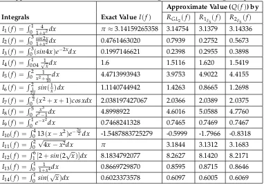
Table 5.1: Comparative study among the quadrature rule RGL2(f),R1F3(f) and R2F3(f)
for approximation of some real definite integrals without using adaptive integration scheme
Approximate Value (Q(f)) by
Integrals Exact ValueI(f) RGL2(f) R1F3(f) R2F3(f)
I1(f) =R011+4x2dx π≈3.14159265358 3.14754 3.1379 3.14336
I2(f) =R03sin1+x2x2dx 0.4761463020 0.7939 0.2752 0.5673
I3(f) =R03(sin4x)e−2xdx 0.1997146621 0.2398 0.2955 0.3898
I4(f) =R0.041 √1xdx 1.6 1.5116 1.620 1.5419
I5(f) =R02x2+11 10
dx 4.4713993943 3.9753 4.9022 4.4155
I6(f) = R2
1 2πsin(
1
x)dx 1.1140744942 1.4263 0.8665 1.2698
I7(f) =R π 2
0 (x2+x+1)cosxdx 2.038197427067 2.0366 2.0389 2.0375
I8(f) =R05 x 3
ex−1dx 4.8998922 4.6016 5.0588 4.7760
I9(f) = R1
0 e−x 2
dx 0.7468241328 0.7465 0.7469 0.7467
I10(f) = R4
0 13(x−x2)e− 3x
2 dx -1.5487883725279 -0.5999 -1.7966 -0.8318
I11(f) = R2
0
√
4x−x2dx π 3.1844 3.1312 3.1683
I12(f) = R6
1[2+sin(2
√
x)]dx 8.1834792077 8.2627 8.1420 8.2171
I13(f) =R011+1x4dx 0.8669729870 0.8595 0.8715 0.8646
I14(f) =R01sin(
√
x)dx 0.6023373578 0.6097 0.6005 0.6069
Table 5.2: Comparative study among the quadrature/mixed quadrature rules (RGL3(f),R2F5(f) and
RGL21F32F3(f)) for approximation of integrals (table 5.1) without using adaptive integration scheme Approximate Value (Q(f)) by
Integrals Exact ValueI(f) RGL3(f) R2F5(f) RGL21F32F3(f)
I1(f) =R011+4x2dx π≈3.14159265358 3.14106 3.14147 3.1415979
I2(f) =R03sin1+x2x2dx 0.4761463020 0.4415 0.4659 0.4751
I3(f) =R03(sin4x)e−2xdx 0.1997146621 0.3913 0.2326 0.1878
I4(f) =R0.041 √1xdx 1.6 1.5667 1.5844 1.5905
I5(f) =R02x2+11 10
dx 4.4713993943 4.6629 4.5628 4.5209
I6(f) =R21 2πsin(
1
x)dx 1.1140744942 1.1304 1.0498 1.0219
I7(f) =R π 2
0 (x2+x+1)cosxdx 2.038197427067 2.03810 2.03817 2.03819762
I8(f) =R05 x 3
ex−1dx 4.8998922 4.8862 4.8968 4.90003
I9(f) =R01e−x 2
dx 0.7468241328 0.746814 0.746822 0.74682421
I10(f) =R0413(x−x2)e− 3x
2 dx -1.5487883725279 -1.1196 -1.43307 -1.5350
I11(f) =R02
√
4x−x2dx π 3.1560 3.1492 3.1468
I12(f) = R6
1[2+sin(2
√
x)]dx 8.1834792077 8.1882 8.1847 8.1836
I13(f) = R1
0 1+1x4dx 0.8669729870 0.8675 0.8670 0.866965
I14(f) =R01sin(
√
x)dx 0.6023373578 0.6048 0.6036 0.6032
Table 5.3: Comparison of the results following from the Gauss-Legendre 2-point rule, Fejer’s first 3-point rule and Fejer’s second 3-point rule for approximating integrals using the adaptive integration scheme
Approximate value (Q(f)) by
Integrals (RGL2(f)) #steps (R1F3(f)) #steps (R2F3(f)) #steps
I1(f) =R011+4x2dx 3.141592690 17 3.141592653573 15 3.14159265359 15
I2(f) = R3
0 sin1+2xx2dx 0.47614627 41 0.476146256 35 0.476146332 35
I3(f) =R03(sin4x)e−2xdx 0.199714693 51 0.199714686 43 0.19971459 39
I4(f) =R0.041 √1xdx 1.59999986 39 1.6000001 35 1.59999986 31
I5(f) =R02x2+1101 dx 4.471399346 53 4.471399461 49 4.471399326 43
I6(f) =R21 2πsin(
1
x)dx 1.114074589 51 1.114074448 43 1.114074503 41
I7(f) =R π 2
0 (x2+x+1)cosxdx 2.0381974132 23 2.0381974183 17 2.0381974106 15
I8(f) =R05 x 3
ex−1dx 4.899892102 43 4.899892237 39 4.899892026 29
I9(f) =R01e−x 2
dx 0.7468241276 15 0.746824114 13 0.746824120 11
I10(f) =R0413(x−x2)e− 3x
2 dx -1.5487882018 57 -1.5487884508 51 -1.5487882663 47
I11(f) =R02
√
4x−x2dx 3.1415929475 45 3.141592395 37 3.141592855 39
I12(f) =R16[2+sin(2
√
x)]dx 8.1834793329 31 8.18347908 27 8.183479317 25
I13(f) = R1
0 1+1x4dx 0.8669729661 15 0.86697299 15 0.866972942 13
I14(f) =R01sin(
√
x)dx 0.602337696 29 0.602337112 25 0.602337592 25
N:B:The prescribed tolerance(e)=0.000001
Table 5.4: Comparison of the results following from the Gauss-Legendre
3-point rule, Fejer’s second 5-point rule and mixed quadrature rule RGL21F32F3(f) for
approximating integrals (given in table 5.3) using the adaptive integration scheme
Approximate Value (Q(f)) by
Integrals (RGL3(f)) #steps (R2F5(f)) # steps (RGL21F32F3(f)) #steps
I1(f) = R1
0 1+4x2dx 3.14159265347 7 3.141592651 3 3.141592653589621 3
I2(f) =R031sin+2xx2dx 0.4761463032 15 0.4761463085 11 0.4761463008 5
I3(f) =R03(sin4x)e−2xdx 0.1997146667 19 0.1997146587 13 0.1997146616 9
I4(f) =R0.041 √1xdx 1.599999987 17 1.599999985 13 1.599999998 9
I5(f) =R02x2+11 10
dx 4.4713993946 17 4.471399387 15 4.471399396 11
I6(f) =R21 2πsin
(1x)dx 1.114074506 21 1.114074477 19 1.114074495 11
I7(f) =R π 2
0 (x2+x+1)cosxdx 2.0381974267 7 2.0381974227 3 2.03819742776 1
I8(f) =R05 x 3
ex−1dx 4.8998921534 13 4.8998921579 7 4.899892158 3
I9(f) =R01e−x 2
dx 0.7468241324 3 0.7468241327 3 0.7468241329 1
I10(f) =R0413(x−x2)e− 3x
2 dx -1.5487883665 21 -1.548788353 13 -1.5487883721 9
I11(f) =R02
√
4x−x2dx 3.1415928159 25 3.1415928990 19 3.141592813 19
I12(f) =R16[2+sin(2
√
x)]dx 8.1834792212 9 8.1834792108 9 8.1834792081 5
I13(f) =R011+1x4dx 0.8669729873 7 0.886972987 7 0.8669729873 3
I14(f) = R1
0 sin(
√
x)dx 0.602337586 17 0.602337475 17 0.60233758 15
N:B:The prescribed tolerance(e)=0.000001
All the computations are done using ‘C’ Program[8].
6
Conclusion
We observe from Tables-5.1 and 5.2, that the mixed quadrature rule gives more accurate result in comparison to their constituent rules. Gauss-Legendre 3-point rule and Fejer’s second 5-point rule when integrals (I1−I14) are evaluated without using adaptive integration scheme. Tables-5.3 and 5.4, reveal that
when these integrals are evaluated using the adaptive integration scheme, the mixed qudrature rule reduces the number of steps to achieve the prescribed accuracy and gives more accurate result in comparison to the their constituent rules, Gauss-Legendre 3-point rule and Fejer’s second 5-point rule.
References
[1] B. Bradie,A Friendly Introduction to Numerical Analysis, Pearson, 2007.
[2] P.J. Davis and P. Rabinowitz,Methods of Numerical Integration, 2nd ed., Academic Press,New York, 1984.
[3] S. Conte, and C.de Boor,Elementary Numerical Analysis, Mc-Grawhill, 1980.
[4] Kendal E Atkinson,An Introduction to Numerical Analysis, 2nd ed., John Wiley, 2001.
[5] R.N. Das and G. Pradhan, A mixed quadrature rule for approximate evaluation of real definite integrals, Int. J. Math. Educ. Sci. Technol., 27(2)(1996), 279-283.
[7] R.B. Dash and D. Das , A mixed quadrature rule by blending Clenshaw-Curtis and Gauss-Legendre quadrature rules for approximation of real definite integrals in adaptive environment,Proceedings of the International Multi-conference of Engineers and Computer Scientists, I(2011), 202-205.
[8] D.Das and R.B.Dash, Application of mixed quadrature rules in the adaptive quadrature routine,General Mathematics Notes (GMN), 18(1)(2013), 46-63.
[9] D. Das and R. B. Dash, Numerical computation of integrals with singularity in the adaptive integration scheme involving a mixed quadrature rule,Bulletin of Pure and Applied Sciences, 32E(1)(2013), 29-38.
[10] R.B. Dash and D. Das, Identification of some Clenshaw-Curtis quadrature rules as mixed quadrature of Fejer and Newton-Cotes type of rules,Int. J. of Mathematical Sciences and Applications, 1(3)(2011), 1493-1496.
[11] A.K.Tripathy, R.B.Dash and A. Baral, A mixed quadrature rule blending Lobatto and Gauss-Legendre three-point rule for approximate evaluation of real definite integrals, Int.J. Computing science and Mathematics, Accepted for publication.
Received: October 10, 2014;Accepted: May 23, 2015
UNIVERSITY PRESS