Copyright © The Author(s). All Rights Reserved. Published by American Research Institute for Policy Development DOI: 10.15640/jeds.v5n3a12 URL: https://doi.org/10.15640/jeds.v5n3a12
Consumption and Saving: Another Glance at the Life Cycle Framework
Nor Azam Abdul Razak
1, Roslan Abdul Hakim
2Abstract
This paper investigates the behavior of consumption and saving in Malaysia from the perspective of the life cycle hypothesis (LCH). Specifically, the analysis employs the Deaton-Paxson model which decomposes the pattern of household consumption and saving into age effects and cohort effects. Using the household data from three Household Expenditure Surveys of Malaysia, this study produces two key results. First, the age effects of income and consumption rise with age but the latter rise more rapidly; thus, the age effects of saving fallwith age. This set of results suggests that individuals engage in a lifetime saving plan early in their working lives (which is consistent with the prediction of LCH); yet, their saving falls gradually over time and approaches zero (instead of becoming negative) toward the end of their lifetime (inconsistent with the prediction of LCH). Second, the cohort effects of income and consumption fall with cohort but the latter fall more rapidly; hence, the cohort effects of saving rise with cohort. This set of results suggests that economic boom generates an unwarranted optimism in that individuals choose to consume at the expense saving; therefore, growth stimulates consumption instead of saving (inconsistent with the prediction of LCH). Keywords: life cycle hypothesis, consumption, saving, age effects, cohort effects.
JEL Codes: D12, D91, E21, O11. 1. Introduction
Consider a fresh college graduate who has recently assumed an entry-level management position in a manufacturing firm in his neighborhood. Being a man of reasonable vision and competence, he expects to move up the career ladder in a fairly progressive manner: becoming a junior middle-level manager in the next five years, a senior middle-level manager in the next 10 years, and eventually a top-level manager in the next 10 years (until his retirement in the next 10 years). It goes without saying that this four-stage career progression (along with the annual salary increments) would ensure a steady and generous increase in his income up to his retirement.
What is the likely lifestyle of a person characterized by this type of career path and income level? According to the life cycle theory of consumption and saving (Modigliani & Brumberg, 1954, 1980; and Modigliani & Ando, 1963), a rational and forward-looking individual maximizes his expected lifetime utility subject to his lifetime budget constraint. Such intertemporal optimization problem yields a key prediction that one‟s consumption is proportional to one‟s expected lifetime income (as opposed to one‟s current income as allegedly conjectured by Keynes). Because one‟s lifetime income is spread evenly over his lifetime, one‟s consumption turns out to be a fraction of his lifetime income, which implies a constant age profile of consumption. In the life cycle literature, this consumption behavior is known as consumption smoothing.
1 School of Economics, Finance & Banking, Universiti Utara Malaysia. E-mail: [email protected]
Because one‟s income is expected to rise throughout his working years and drop abruptly upon his retirement, we would expect to see a hump-shaped age profile of income. Taken one‟s consumption and income behavior together, we observe the following: initially, one‟s income would be outstripped by his consumption; over time, his consumption would be outstripped by his income; upon retirement, his income would be outstripped by his consumption again. Inasmuch as saving is the difference between income and consumption, it follows that saving is negative initially, positive subsequently, and negative again upon retirement (see Attanasio& Weber, 2010; and Browning & Crossley, 2001).
Do people behave this way in terms of consumption and saving? Since the inception of the life cycle theory in the mid-1950s and its refinements in the next few decades, many attempts have been made to test the implication of consumption smoothing. The test is based on the idea that, since one‟s consumption is a function of one‟s lifetime income instead of current income, there should be no evidence of consumption-tracking-income behavior. In many empirical studies, unfortunately, scholars find that there is such evidence, thereby casting doubt on the validity of the theory (see, for example, Campbell & Mankiw, 1990; Carroll & Summers, 1991; and Deaton &Paxson, 1994).
In this paper, another attempt to validate the theory is made in the context of a developing country, Malaysia. Our point of departure is a simple model of consumption and saving developed and applied by Deaton andPaxson (1994) and subsequently applied by Paxson (1996) and Alba and See (2006), to name a few. Besides its simplicity, this model is chosen for its two remarkable features: a) its ability to test the consumption-tracking-income behavior using the called age effects, and b) its ability to test the link between economic growth and aggregate saving using the so-called cohort effects.
A common feature of these studies is that they are based on the household data which are compiled from the annual or periodic surveys of household income and expenditures in individual countries. Deaton andPaxson (1994) employed the household data from the Personal Income Distribution Survey in Taiwan during the period 1976-1990. Paxson (1996) used the household data from two developed countries (the U.S. and U.K.) and two developing countries (Taiwan and Thailand). For the U.S., the data came from the Consumer Expenditure Survey during the period 1980-1992. For the U.K., the data came from the Family Expenditure Survey during the period 1970-1992. For Thailand, the data came from the Socio-Economic Survey during the period 1976-1992. For Taiwan, the data were extracted from Deaton and Paxson (1994). Alba and See (2006) utilized the household data from the Family Income and Expenditures
Survey in the Philippines during the period 1988-2000. Of these surveys, some were annual (that is, Taiwan, the U.S.,
and the U.K.) while others were periodic (that is, Thailand and the Philippines). For Thailand, the surveys were conducted in 1976, 1981, 1986, 1988, 1990, and 1992; for the Philippines, the surveys were conducted in 1988, 1991, 1994, 1997, and 2000.
2. A Preliminary Look at the Data
In this paper, we employ the household data from the Household Expenditure Survey in Malaysia during the period 1988-2010.However, the surveys were spaced roughly five years apart; in particular, the surveys were conducted in 1998/1999, 2004/2005, and 2009/2010. The number of households (or the sample size) varies from one survey to another, ranging from 8,000- to 19,000-odd observations. For each survey, however, the data sets of only one-third of the actual sample are made available to the researchers; hence, 2761, 4225, and 6495 in the first, second, and third surveys, respectively.
Each survey contains the data on income, expenditures, and demographic characteristics of the households. The income data are divided into several categories of earnings such as wage income, self-employed income, and property income. The expenditure data are divided into several major categories (nine in the first survey and 12 in the other two surveys) which, in turn, are further divided into several subcategories, up to six digits. The demographic data are divided into household- and individual-level data. At the household level, the available data include household size, number of income earners, number of dependents, and residential type. At the individual level, the available data include age, gender, ethnicity, education level, and occupation type of the household head (HHH) and members.
When it comes to the expenditure data alone, it should be noted that some additional data processing needs to be made. Basically, this data processing involves two tasks. The first task is to reshuffle the nine major expenditure categories in the first survey to match the 12 major expenditure categories in the other two surveys. This discrepancy reflects the fact that certain expenditure items which are decomposed into two categories in the other two surveys are lumped together into one category in the first survey (see Table 1). For comparability, we disaggregate the expenditure items in the first survey to match those in the other two.
Table 1: Major Categories of Household Expenditures
No. 1998/1999 No. 2004/2005 and 2009/2010 1 Food and Non-alcoholic Beverages 1 Food and Non-alcoholic Beverages 2 Alcoholic Beverages and Tobacco 2 Alcoholic Beverages and Tobacco 3 Clothing and Footwear 3 Clothing and Footwear
4 House Rent and Utilities 4 House Rent and Utilities 5 House Furnishings, Equipment
and Maintenance 5 House Furnishings, Equipment and Maintenance 6 Medical Care and Health 6 Medical Care and Health 7 Transportation and Communication 7 Transportation
8 Communication 8 Recreation, Entertainment, Culture
Services and Education 9 Recreation, Entertainment and Cultural Services 10 Education
11 Restaurants and Hotels
9 Miscellaneous Goods and Services 12 Miscellaneous Goods and Services
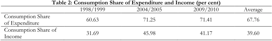
The second task is to derive the data on household consumption. This is accomplished by subtracting certain expenditure items that are not usually regarded as consumption from the original expenditure data. These items include mortgage payments (which are regarded as residential investment), expenditures on durable goods (which are regarded as physical capital investment), education and health expenses (which are regarded as human capital investment), and insurance payments (which are regarded as a form of saving)(see Attanasio, 1998). Once this is done, we find that household consumption constitutes an average of about 68per cent of the household expenditures and 40per cent of the household income (see Table 2). Thus, household saving constitutes an average of about 60per cent of the household income.
Table 2: Consumption Share of Expenditure and Income (per cent)
1998/1999 2004/2005 2009/2010 Average Consumption Share
of Expenditure 60.63 71.25 71.41 67.76
Consumption Share of
Income 31.69 45.98 41.17 39.60
A remarkable feature of the household survey data is that they are not of panel type, where the same groups of households are tracked over time. Instead, the data constitute a few time series of cross-sectional type. With this type of data, the best one can do is to construct a synthetic (or pseudo-) panel data based on the cohorts of households, and subsequently make an inference on the household consumption based on these household cohorts. 3. Constructing the Cohort Data
Table 3: The Distribution of Households
Age 1998/1999 2004/2005 2009/2010
15 – 19 37 28 34
20 – 24 117 140 192
25 – 29 241 295 534
30 – 34 284 408 668
35 – 39 383 525 818
40 – 44 398 597 868
45 – 49 331 572 917
50 – 54 275 478 769
55 – 59 234 364 596
60 – 64 174 275 406
65 – 69 126 237 304
70 – 74 78 141 205
75 – 79 38 77 102
80 26 83 67
Total 2742 4223 6480
Note: Age refers to the HHH‟s age at the time of the survey. For each survey, the number of households is less than what was stated earlier due to the missing values on the age of some HHHs.
In the LCH literature, it is typical to define the household cohorts by the age of HHH in a given year during the sample period (Browning et al., 1985). In view of the fact that the three surveys were spaced roughly five years apart and in order to ensure that the cohorts became 5 and 10 years older in the second and third surveys, respectively, let us define the cohorts based on the HHH‟s age in 1999. Specifically, let the first cohort be defined as the group of households whose HHHs aged 20-24 in 1999 (so that it became 25-29 in 2004, and 30-34 in 2009); the second cohort as the one whose HHHs aged 25-29 in 1999 (so that it became 30-34 in 2004, and 35-39 in 2009); and so on until the tenth cohort as the one whose HHHs aged 65-69 in 1999 (so that it became 70-74 in 2004, and 75-79 in 2009). Then, the distribution of household cohorts in all of the three surveys can be depicted as in Table 4. A glance at the table indicates that the size of household cohorts varies from as small as 105 (the 10th cohort in 2009/2010) to as large as 896 (the fourth cohort in 2009/2010).
Table 4: The Distribution of Household Cohorts
Cohort Age1999 1998/1999 2004/2005 2009/2010
1 20 – 24 117 296 668
2 25 – 29 228 409 832
3 30 – 34 282 526 857
4 35 – 39 368 588 896
5 40 – 44 405 575 792
6 45 – 49 338 485 597
7 50 – 54 288 366 412
8 55 – 59 229 278 308
9 60 – 64 180 226 208
10 65 – 69 130 141 105
Total 2565 3890 5675
Note: Age1999 refers to the HHH‟s age in 1999.
Given the 10 cohorts and three periods of observations, the cohort data to be generated will have 30 observations only. If we wish to increase the sample size, we need to redefine the cohort on a higher frequency basis, say, on an annual basis. Doing so increases the number of cohorts to 50 and we end up with 150 observations. However, the increase in the sample size comes at the expense of the cohort size.
The low cohort size is a cause of concern since there might be insufficient variation in the data to generate acceptable cohort means (Browning et al., 1985).
4. Model Specification
In this paper, we follow the model of consumption and saving developed by Deaton andPaxson (1994) by stipulating that an individual‟s consumption is a function of the interaction between his preferences and lifetime wealth. One‟s preferences reflect one‟s needs, which evolve according to one‟s stage in the life cycle (that is, getting a job, getting married, having children, and so forth). Hence, one‟s preferences vary according to changes in his demographic characteristics such as age, household size, and household composition. One‟s lifetime wealth reflects one‟s accumulated income plus bequests (if any) throughout his working life.
Table 5: The Distribution of Household Cohorts
Cohort Age1999 1998/1999 2004/2005 2009/2010
1 20 21 45 142
2 21 19 49 124
3 22 20 63 141
4 23 24 72 124
5 24 33 67 137
6 25 30 67 159
7 26 40 69 160
8 27 49 91 167
9 28 50 87 156
10 29 59 95 190
11 30 50 107 175
12 31 52 99 161
13 32 50 95 192
14 33 65 108 155
15 34 65 117 174
16 35 62 127 171
17 36 74 105 173
18 37 74 110 182
19 38 73 128 177
20 39 85 119 193
21 40 88 116 193
22 41 84 112 146
23 42 81 137 145
24 43 80 116 177
25 44 72 94 131
26 45 75 126 144
27 46 69 98 135
28 47 63 91 117
29 48 62 86 92
30 49 69 83 109
31 50 64 85 108
32 51 72 81 67
33 52 62 71 94
34 53 46 67 67
35 54 44 62 76
36 55 44 54 64
37 56 51 53 58
38 57 41 55 72
39 58 52 57 57
40 59 41 59 57
41 60 44 51 57
42 61 36 59 38
43 62 53 48 45
44 63 25 41 34
45 64 22 27 34
46 65 35 39 29
48 67 23 32 16
49 68 14 23 21
50 69 21 18 19
Total 2565 3890 5675
Note: Age1999 refers to the HHH‟s age in 1999.
From the modelling point of view, a key difference between the two is that while one‟s preferences vary over time, one‟s lifetime wealth is fixed over time. (Nonetheless, both variables vary across individuals.) Hence, a simple model of consumption can be expressed as follows:
,
(.) ij
it
ijt W
c
(1)where cijt denotes the consumption of individual i of cohort j at time t, it(.) the preference function of individual i at time t, and Wij the lifetime wealth of individual i of cohort j. Note that one‟s preferencesvary across individuals and time but not across cohorts while one‟s wealth varies across individuals and cohorts but not across time.
The multiplicative nature of the right-hand-side variables suggests that they can be decomposed by taking logarithms, yielding:
. ln (.) ln
lncijt
it Wij (2)One conceptual issue related to working with the cohort data is that the consumption data are available at the household (instead of individual) level. This problem is usually assumed away by treating households and individuals interchangeably (that is, i may refer to a household as well as an individual). This paper shall do the same (for an alternative treatment, see Deaton & Paxson, 2000).
Another conceptual issue related to working with the cohort data is the inability to track the same households over time. As Browning et al. (1985) put it, the best we can do is to track the same cohorts of households over time. In the LCH literature (see Deaton &Paxson (1994) and Paxson (1996)), this is accomplished by identifying the cohorts by the ages of household head (HHH) and averaging over all households which belong to the same cohorts, yielding:
.
ln
(.)
ln
ln
c
jt
t
W
j (3)where the left-hand-side variable is the cohort average of the log of household consumption; that is,
,
ln
ln
1 1
j j N i ijt N jtc
c
where Nj is the size of cohortj (for example, for the first cohort, there 21, 45, and 142 households for the three consecutive surveys; hence, N1 = 21 in the first survey, N1 = 45 in the second survey, and N1 = 142 in the third survey).Consider the second variable on the right-hand side of Eq.(3). Since the variable reflects household‟s lifetime wealth, which may vary across individuals and cohorts but not over time, it can be captured by the cohorts of households (see Deaton &Paxson (1994) and Paxson (1996)). Thus, a set of cohort dummies can be defined as follows:
.
otherwise
0
69
if
1
...;
;
otherwise
0
21
if
1
;
otherwise
0
20
if
1
99 50 99 2 99 1
age
COH
age
COH
age
COH
(4)Now consider the first variable on the right-hand side of Eq.(3). Since the variable reflects household‟s preferences, which may vary across individuals and over time but not across cohort, t can be captured by the HHH‟s age (see Deaton &Paxson (1994) and Paxson (1996)). Hence, a set of age dummies can be defined as follows:
.
otherwise
0
79
if
1
...;
;
otherwise
0
21
if
1
;
otherwise
0
20
if
1
60 2 1
t tage
tAGE
age
AGE
age
AGE
(5)Note that aget refers to the HHH‟s age at the time of the survey and age99 the HHH‟s age in 1999. Given the definitions of age and cohort dummies, Eq.(3) can be written as
60 50,
where t is the current year, a is the index of HHH‟s age, j is the index of household cohort, S is the average household size, 1, 1‟s, and 1„s, and are parameters, and u1 is the error term.
Eq.(6) indicates that consumption of the 10 cohorts of households can be decomposed into two terms: age effects and cohort effects (Deaton &Paxson, 1994). The difference between the two is that the age effects measure the effects of the lifetime preferences of the same cohort of households on consumption, whereas the cohort effects measure the effects of the lifetime wealth of the different cohorts of households on consumption.
To illustrate, suppose we pick a 21-year-old HHH in 2000. Obviously, he belongs to the second age group, AGE2, in 2000. If we track this person over time, we see that he moves to AGE7 in 2005, to AGE12 in 2010, and so on. Since he was 20 years old in 1999, however, he will always be in the first cohort group, COH1. Thus, holding the cohort constant, the age effects measure the effects of the lifetime preferences of the same cohort of households on consumption.
Now suppose we pick a 32-year-old HHH in 2010. Since he must have been 21 years old in 1999, he must belong to COH2. If we pick another 32-year-old HHH in 2005, he must have been 26 years old in 1999; thus, he must belong to COH7. If we pick still another 32-year-old HHH in 2000, he must have been 31 years old in 1999; thus, he must belong to COH12. Needless to say, all of them belong to the thirteenth age group, AGE13. Thus, holding the age fixed, the cohort effects measure the effects of the lifetime wealth of the different cohorts of households on consumption. In order to determine whether the pattern of household consumption mirrors that of household income, we specify and estimate the corresponding income function as follows:
,
ln
50 21 2 60
1 2
2
AGE
COH
S
u
y
jj j j
a a t
jt
(7)where the left-hand-side variable is the cohort average of the log of household income. Other variables and parameters are as defined before.
Inasmuch as the saving rate is approximately equal to the difference between the cohort average of the log of household income and that of household consumption,
s
y
ln
y
jt
ln
c
jt,
the pattern of household saving can beresidually calculated.
From the perspective of LCH, the age effects of consumption are relatively flat (due to consumption-smoothing behavior) while the age effects of saving are hump-shaped (because individuals borrow (or save little) when they begin employment, save (or increase their saving) as they mature, and dissave during their old age). In the face of a growing economy, the cohort effects of consumption, income, and saving are downward-sloping because the younger cohorts are relatively wealthier than the older ones.
5. Empirical Analysis
Given the household data in Malaysia for a sample of 50 cohorts observed every five years during the period 1998-2010, we estimate the models in Eqs.(6)–(7) using the OLS method.
Because we are interested in examining the age effects and the cohort effects on consumption and income, the joint tests of significance of the corresponding effects are conducted. For consumption, the joint tests of significance of the age effects and the cohort effects are determined by testing whether H0: 1,1 = 1,2 = … = 1,59 = 0
and H0: 1,1 = 1,2 = … = 1,49 = 0, respectively, can be rejected (and likewise for income). As shown in Table 6, the
age effects and cohort effects on consumption and income are jointly significant at the 1% level.
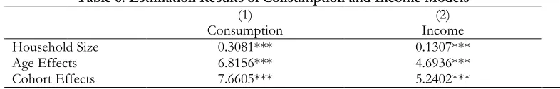
Table 6: Estimation Results of Consumption and Income Models
(1)
Consumption Income (2) Household Size 0.3081*** 0.1307*** Age Effects 6.8156*** 4.6936*** Cohort Effects 7.6605*** 5.2402***
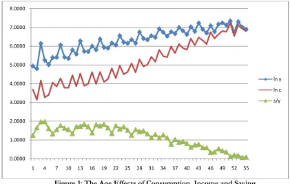
In order to examine the pattern of the age effects on consumption, income, and saving, we plot the estimated coefficients of the age dummies from each of the above regressions. Figure 1 shows that the age effects are sloping upward for both income and consumption, signifying that both of them are rising with age. What is intriguing is that the age effects of consumption are steeper than the age effects of income, allowing them to converge toward the end of one‟s lifetime. As a consequence, the age effects of saving (which are residually derived) are declining with age. Given these profiles, it follows that one starts to save very dearly as soon as one begins one‟s employment; over time, however, one‟s consumption quickly catches up with one‟s income so that saving is exhausted toward the end of one‟s lifetime. Apparently, this story does not fit well into the standard life cycle model: consumption converges to income (instead of remaining flat), saving converges to zero (instead of becoming negative) toward the end of one‟s lifetime, and income continues to be positive (instead of falling to zero) beyond the retirement age.
Figure 1: The Age Effects of Consumption, Income and Saving
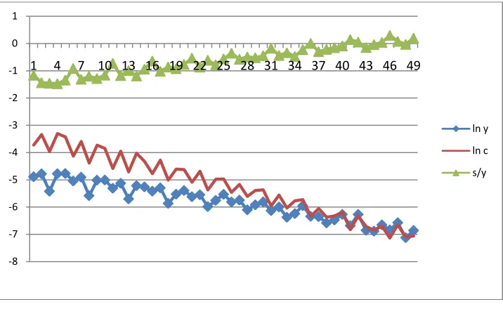
In order to examine the pattern of the cohort effects on consumption, income, and saving, we plot the estimated coefficients of the cohort dummies from each of the above regressions. Figure 2 shows that the cohort effects are sloping downward for both income and consumption, indicating that the younger cohorts are wealthier (which is hardly surprising for a growing economy) and therefore consume more than the older cohorts (which is hardly surprising across cohorts). What is perplexing is that the cohort effects of consumption are steeper than the cohort effects of income, allowing them to converge toward the oldest cohort. As a result, the cohort effects of saving are rising with cohort. Given these profiles, it follows that as the economy grows over time, one forms an expectation that it will continue to grow; thus, one tends to consume the “extra income” at the expense of saving. Obviously, this optimistic behavior does not fit well into the standard life cycle model: in the face of a rapid economic growth, the younger cohorts consume at the expense of saving; hence, economic growth stimulates consumption instead of saving.
0.0000 1.0000 2.0000 3.0000 4.0000 5.0000 6.0000 7.0000 8.0000
1 4 7 10 13 16 19 22 25 28 31 34 37 40 43 46 49 52 55
Figure 2: The Cohort Effects of Consumption, Income and Saving 6. Conclusion
In this paper, we reexamine the behavior of consumption and saving from the perspective of the life cycle hypothesis. In particular, we employ a simple model of consumption and saving developed by Deaton andPaxson (1994) which decomposes the pattern of household consumption and saving into the age effects and cohort effects. Using a sample of 50 cohorts of households in Malaysia which are tracked every five years during the period 1998-2010, we estimate the age effects and cohort effects on consumption and income (and residually calculate the age effects and cohort effects on saving). We find that both the age effects and cohort effects for each consumption and income regression are jointly significant. Graphically, we observe the following two sets of results. First, the age effects of income and consumption are rising with age but the latter is rising more rapidly; thus, the age effects of saving are falling with age. Second, the cohort effects of income and consumption are falling with cohort but the latter is falling more rapidly; hence, the cohort effects of saving are rising with cohort. The first set of results implies that individuals engage in a lifetime saving plan early in their working lives (which is consistent with the prediction of the life cycle hypothesis); yet, their saving gradually falls over time and approaching zero toward the end of their lifetime (which is inconsistent with the prediction of the life cycle hypothesis). The second set of results implies that economic boom generates an unwarranted optimism in that individuals choose to consume at the expense saving; therefore, growth stimulates consumption instead of saving (which is consistent with the prediction of the life cycle hypothesis). Acknowledgments:
This work was supported by the Fundamental Research Grant Scheme (FRGS) No. 12350 provided by the Ministry of Higher Education of Malaysia.
References
Alba, M. and See, E. (2006). Exploring Household Saving and Consumption-Smoothing in the Philippines. Philippine
Journal of Development, 33 (1 and 2): 7799.
Attanasio, O. and Weber, G. (2010). Consumption and Saving: Models of Intertemporal Allocation and Their Implications for Public Policy. Journal of Economic Literature, 48: 693751.
Attanasio, O. (1998). Cohort Analysis of Saving Behavior by U.S. households. Journal of Human Resources, 33 (3): 575609.
Browning, M, Deaton, A., and Irish, M. (1985). A Profitable Approach to Labor Supply and Commodity Demands over the Life Cycle. Econometrica, 53: 503544.
Browning, M. and Crossley, T. (2001). The Life-Cycle Model of Consumption and Saving. Journal of Economic
Perspectives, 15 (3): 322.
-8 -7 -6 -5 -4 -3 -2 -1 0 1
1 4 7 10 13 16 19 22 25 28 31 34 37 40 43 46 49
Campbell, J. and Mankiw, N. G. (1990). Consumption, Income, and Interest Rates: Reinterpreting the Time Series Evidence. National Bureau of Economic Research Working Paper #2924.
Carroll, C. andSummers, L. (1991). Consumption Growth Parallels Income Growth: Some New Evidence, in B. D. Bernheim and J. B. Shoven (ed), National Saving and Economic Performance. Chicago: Chicago University Press. Deaton, A. andPaxson, C. (1994). Saving, Growth and Aging in Taiwan, in David A. Wise (ed), Studies in the Economics
of Aging. Chicago: Chicago University Press.
Deaton, A. andPaxson, C. (2000). Growth and Saving among Individuals and Households. Review of Economics and
Statistics, 82 (2): 212225.
Modigliani, F. and Ando, (1963). The Life Cycle Hypothesis of Saving: Aggregate Implications and Tests. American
Economic Review, 53:5584.
Modigliani, F. andBrumberg, R. (1954). Utility analysis and the Consumption Function: An Interpretation of Cross-Section Data, in K. K. Kurihara (ed), Post Keynesian Economics. New Brunswisk: Rutgers University Press. Modigliani, F. andBrumberg, R. (1980). Utility Analysis and the Consumption Function: An Attempt at Integration, in
Andrew Abel (ed), The Collected Papers of Franco Modigliani: The Life Cycle Hypothesis of Saving. Cambridge: Cambridge University Press.