The Application of Liquid State Machines in
Robot Path Planning
Zhang Yanduo
School of Computer Science and Engineering, Wuhan Institute of Technology, Wuhan, Hubei, China
Wang Kun
School of Computer Science and Engineering, Wuhan Institute of Technology, Wuhan, Hubei, China
Abstract – This paper discusses the Liquid state machines and does some researches on spiking neural network and Parallel Delta Rule, using them to solve the robot path planning optimization problems, at the same time we do simulation by Matlab, the result of the experimental reveal that the LSM can solve these problems effectively.
Index Terms - Liquid state machines; spiking neural networks; Parallel Delta Rule; path planning
I.INTRODUCTION
The liquid state machines[1] is a kind of new recurrent neural network proposed by Maass, which has a similar concept with echo state machines[2] proposed by Jaeger. Sometimes, general recurrent neural network will meet some troubles in solving practical problems, for example, on the problem of training convergence it can't find a sufficient fast convergence training method when the neural network requires a strong convergence, and it can't approach the nonlinear systems in some nonlinear projection. But the LSM isn't the same as general recurrent neural network, which can do real-time calculation for continues input-flow, the process is to put input-flow into a large enough complex recurrent neural network, because the network itself has a dynamic characteristic, which can translate a lower-resolution input information into 'liquid' or 'echo' state owning a higher-resolution, while this state is difficult to understand, we can extract information using a special output unit. Through those features, the LSM can do better in approaching nonlinear systems, which cause to obtain a better result in many nonlinear forecasting. This paper mainly discusses how to using the LSM to solve the robot path planning such a complicated nonlinear problems.
In the mobile robot technology research, navigation technology is the core, and the path planning is an important part of the study and the subject to navigation research. The path planning is: when the mobile robots
move along one path from an initial position to another target position, designing an appropriate path so that the robots can be safe and collision-free to bypass all obstacles in the movement process.
II.LIQUID STATE MACHINES
Liquid state machines can be best explained by the following example: imagine a rock and a pond and throw the rock into the water. In fact, here the rock is a low-dimensional temporal input: the rock and throw have some properties but these are only expressed very briefly. The resulting splash and ripples that are created can be seen as the reaction, or ‘liquid’ state. These ripples propagate over the water’s surface for a while and will interact with the ripples caused by other recent events. The water can thus be said to retain and integrate information about recent events, so if we’re somehow able to ‘read’ the water’s surface we can extract information about what has been recently going on in this pond. We refer to this trained spectator as a readout unit that we can ask at any one time what’s going on in the pond, provided that we can show him a picture of the water’s surface.
Formally, the LSM works as follows[3,4]: A continuous input stream
u
( )
⋅
of disturbances is injected into excitable medium LM that acts as a liquid filter. This liquid can be virtually anything from which we can readit’s current liquid state
( )
M
X
t
at each time step t. This liquid state is mapped to target output function
y t
( )
by means of a memory-less readout functionM
f
Figure 1 LSM’s structure
The most important aspect of the liquid is to react differently enough to different input sequences. The amount of distance created between those is called the separation property (SP) of the liquid. The SP (see fig. 2) reflects the ability of the liquid to create different trajectories of internal states for each of the input classes. The ability of the readout units to distinguish these trajectories, generalize and relate them to the desired outputs is called the approximation property (AP). This property depends on the adaptability of the chosen readout units, whereas the SP is based directly on the liquid’s complexity.
Figure.2. The separation property of a generic neural microcircuit, a randomly generated LSM Plotted on the y-axis is the distance between the two states of the liquid in reaction to input signals that have
Euclidian distance
d u v
( , )
By using biologically sufficiently realistic neural networks as micro-columns in the liquid we might both be able to tap the power of the cortical microcircuits, while at the same time learning a fair bit about the capabilities of their biological counterparts. Maass used randomly generated networks of 135 spiking neurons per column and used biological data to define parameters like connectivity, synaptic efficacy and membrane time constants. He used spike trains as input and those are fed to a random 20% of the neurons in the network. It remains a question how the level of realism relates to the computational abilities of these microcircuits.
Recapitulating, the basic action in the liquid state machine is the transformation and integration of continuous low-dimensional input streams into perturbations of the higher dimensional liquid to facilitate feature extraction[5]. The internal dynamics ensure that the current state of the liquid will hold information about recent inputs. The high-dimensionality of this liquid state helps making recognition much easier. First of all, during the memory-span of the liquid the complex low-dimensional temporal problem is turned into a more uid, the complex low-dimensional temporal problem is turned into a more easily solvable spatial recognition task. Secondly, the high dimensionality and dynamics make it theoretically virtually impossible that two different inputs lead to exactly the same network state or state trajectory. In fact, inputs that are radically different are likely to lead to vastly different states of the liquid: allowing the readout units much easier discrimination.
III.ROBOT PATH PLANNING
In moving robot working conditions, the obstacle approaches with the convex polyhedron (e.g. cuboid), a non-convex polyhedron may be expressed with the combinations of several convex polyhedrons.
Figure 3 single obstacle model
The figure3 gave a cuboid represented the obstacle and its six inequality constraints. Know by figure3, through judging a spot’s coordinate whether simultaneously to satisfy six inequalities’ requests to know whether this spot is located in the obstacle, the spatial point
( ,
, )
i i i ip x y z
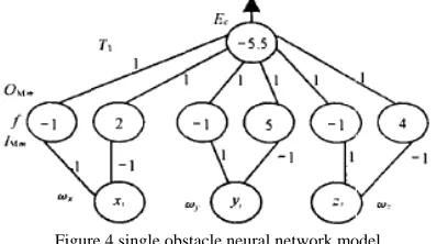
and obstacle cuboid's position can be expressed with the neural network model shown in Figure 4.
Figure 4 single obstacle neural network model
coordinate assigned the way
x
i,y
i ,z
i, the toplayer node's output expresses the obstacle’s collision punishes function (collision punishes function expresses the collision degree quantification between path point and obstacle), the mediate layer node's threshold value expresses the constant item in inequality, from the mediate layer to the top layer the connection scaling coefficient are 1, from input layer to mediate layer the connection scaling coefficient are the variable
x
,y
,z
coefficient in inequality, the top layer node'sthreshold value takes subtracts 0.5 after the inequality integer the negative number.
Neural network's operation relations are:
1
( )
c
=
f T
1 1 G
Mm o m
T
O
ϑ
=
=
∑
+
(
)
Mm Mm
O
=
f I
Mm xm i ym i zm i Mm
I
=
w x
+
w y
+
w z
+
ϑ
Above all formulas, c is the top layer node output;
T
1is the top layer node input;
ϑ
o is the top layer nodethreshold value;
O
Mm is the mediate layer them
thnode output;
I
Mm is the mediate layer them
th nodeinput;
ϑ
Mm is the mediate layerm
th node thresholdvalue;
w
xm,w
ym,
w
zmarem
th the inequality limitedcondition coefficient.
IV.THE LSMPRACTICAL APPLICATION
The only difference between the LSM and the echo state neural network is that the LSM neurons are spiking neurons, and the echo state neural network are general neurons.
Spiking neurons model [6] is a mathematical model
which is closer to the biological neurons. The traditional Sigmoid neurons model is that through a transfer function convert a real input into a real output signal, and through synaptic links transmit this output signal to other connected neurons, this conversion between input and output is one to one, while Spiking neurons model is different which is a spike events converter, when spike neurons receive external stimuli (external input and father synapse neurons input) which cause membrane voltage exceed threshold, the spike neuron will produce a spike and send a output signal, known as the post-synaptic potential, referred to as the PSP.
Spike response model (referred to as SRM) and Integrate-and-fire Model are common neuron models, which are threshold sent model. Integrate-and-fire Model simulated the Hodgkin-Huxley model, and be better to obtain nervous system’s dynamic nature, it is mainly used in this paper.
The LSM’s input layer is equal to a buffer memory, it
added the data source to the network, its nodes number are depended on the data sources dimension that is the dimension of the feature vector. We should consider the vector chose that gives a full description on things essential character When we choice the feature vector. Of course, how to select the feature vector is not what the more dimension is and the better is, the increased feature vector dimension will cause the network calculation appeared exponential growth and lead to an explosion. So, we should consider the reality to select the appropriate the feature vector to reflect the nature characteristics of things. Those good characteristics are: distinguishing, reliability, independence, and a small number.
How to decide the number of output layer nodes, there are certain rules to follow:
1. When the pattern types are few, the output layer nodes equal to the number of pattern types, the m-type outputs by m output units, each output node corresponding to a pattern type, that is, when a output node’s value is 1 and other output nodes are 0, the corresponded input is a particular pattern type sample.
2. When the pattern types are many, using output nodes’ codes to replace all pattern types, that is, the m-type outputs only need m output units.
Following explains the LSM model setup procedure. We suppose that target point is on the right of robot (including the upper right point and right underneath point), the robot walks forward only, cannot retrocede. Has a scale is 100 recurrent neural network stochastically, it has an input level, an output level, inputs the level to have 5 neurons, respectively be on, on right, right, right, the next 5 direction's obstacle to moves robot's distance (to take a maximum range, then carries on normalization to these from value); The output level has 2 outputs, controls robot's running rate and the deflection direction separately.
As the names of both the LSM and ESM hint, there is a resemblance with finite state machines. However, in the finite state machine the full state space and transitions are carefully constructed and clearly defined; quite unlike the rich dynamics found in the medium of an LSM. These state machines could be seen as a universal finite state machine, as a sufficiently highly dynamic ‘liquid’ can implicitly contain the states and transitions of many complex finite state machines. The large advantage of the LSM is that we do not have to define the states themselves, as the readout units can be trained to extract the state from the continuous analog state of the liquid. We only have to make sure that the reaction of the liquid is reliable in the sense that it reaches identifiable states after a predefined number of time steps of input.
satisfactory performance was discovered. Perceptrons compare the summed input received from weighing synapses to a fixed threshold: their output is high if the input is above, or low if it is below this value. They can, however be put to very good use as simple readout units in LSMs. After training with linear regression they can both be applied for classification and for the continuous extraction of information from the liquid state. The presentation of the liquid state to these units is of utmost importance however, especially if both mechanisms speak different ‘languages’: i.e. use pulse and rate coding mechanisms. Though rather simplistic, a low-pass filter can be applied to transform the spike-trains into continuous output that can be weighted and fed to the readout perceptrons. However, there are limitations to the power of linear regression and single perceptrons. Information in the liquid can be encoded in non-linearly separable ways and can thus theoretically not be extracted by these simple readout units. Computationally stronger is the use of perceptrons in pools, using the average activation of all perceptrons as output, or the committee machine. In the latter the Boolean output depends on the majority of the votes in the pool. Still, training these units is complex. Mechanisms that can solve non-linear separable problems in dependable manner are multi-layer perceptrons trained using backprop. These have been successfully applied to extract input timings from low-passed liquid states.
The delta rule is a rule for updating the weights of the neurons in a single-layer perceptron. For a neuron j with activation function
g x
( )
the delta rule for j's ith weightji
w
is given by
'
(
) ( )
ji j j j i
w
α
t
x g h x
∆
=
−
where
α
is a small constant,g x
( )
is theneuron's activation function,
t
j is the target output,x
j is the actual output, andx
j is the ith input. The delta rule is commonly stated in simplified form for a perceptron with a linear activation function as(
)
ji j j i
w
α
t
x x
∆
=
−
The delta rule is derived by attempting to minimize the error in the output of the perceptron through gradient descent. The error for a perceptron with j outputs can be measured as
2
1
(
)
2
j j jE
= ∑
t
−
x
In this case, we wish to move through "weight space" of the neuron (the space of all possible values of all of the neuron's weights) in proportion to the gradient of the error function with respect to each weight. In order to do that, we calculate the partial derivative of the error with respect to each weight. For the ith weight, this derivative can be written as
ji
E
w
δ
δ
Because we are only concerning ourselves with the jth neuron, we can substitute the error formula above while
omitting the
summatio
2 2
1
1
( (
) )
( (
) )
2
j j2
j j jji ji j ij
t
x
t
x
x
E
w
w
x
w
δ
δ
δ
δ
δ
δ
δ
δ
−
−
=
=
'(
j j)
j(
j j)
j j(
j j) ( )
j jij j ij ij
x
x h
h
t x
t x
t x g h
w
h w
w
δ
δ δ
δ
δ
δ δ
δ
= −
=− −
=− −
'(
)
(
) ( )
k jk kj j j
ij
x w
t
x g h
w
δ
δ
= − −
∑
And i ji i jix w
x
w
δ
δ
=
So we get:
'
(
j j) ( )
j i jiE
t
x g h x
w
δ
δ
= − −
As noted above, gradient descent tells us that our change for each weight should be proportional to the
gradient. Choosing a proportionality constant
α
andeliminating the minus sign to enable us to move the weight in the negative direction of the gradient to minimize error, we arrive at our target equation:
'
(
) ( )
ji j j j i
w
α
t
x g h x
∆
=
−
V.SIMULATION RESULT
The LSM 's application could be easily realized with hardware, we usually use CSIM (A neural Circuit SIMulator) in software simulation, which is a kind of tool that can simulate isomerism network constituted by different neurons and the synapses, it is realized in C++ language and can be transferred by matlab with the MEX interaction, it is designed to simulate the network constituted by tens of thousands of neurons (actual size decided by computer's memory).
In CSIM, there are one kind of Learning-Tool, which is established under the LSM's frame, is composed of a series of matlab script language, under this frame, we can simulate LSM. The Circuit-Tools contains a set of Matlab objects and scripts. These objects and scripts allow the multi-‘column’ neural microcircuits construction to be existed with distributed deployed parameters. The neural microcircuit models are simulated by using CSIM.
Leaning-Tool is a tool for analyzing the neural microcircuit models of capability of real-time computing capability. It contains a set of Matlab scripts, and is based on a new theoretical framework which is known as the Liquid State Machine.
1. To ensure that all experiments carried out are fair and adequate, statistical techniques will be employed2. To show a fair comparison between the different algorithms, the same input (randomly generated) will be applied.
3. In order to give a reasonable evaluation, a similar of liquid structure (typically, 3*3*15 spiking neurons) will be used that was used by Maass.
4. To that the user of the system should be able to run the tests with the minimal amount of effort and should be able to control most aspects of the simulation.
5. To gain clearer representations of data and results, graphical representations will be preferred.
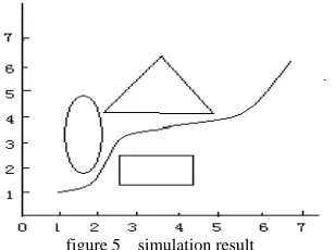
figure 5 simulation result
In the competition of avoiding obstacles in robot football competition, the robot must find the most optimal way from the beginning to the end point in crowd of obstacles, arrive in the shortest time, in the ordinary methods, it is quite difficult to find such a way, but LSM could solve this question very well, there are the simulation result chart above, if it is realized with the hardware, then it might be used in the actual competition.
VI.CONCLUSION
After software simulation, LSM could be realized by the hardware conveniently, which has practical significance, this article simply introduced the LSM's general concept, by which we effectively solved the problem of moving robot's way plan, the experimental result indicated that it could produce optimal way without collision effectively and fast.
REFERENCES
[1] Maass,W. Natschlager,T&Markram,H. Real-time computing without stable states: A new framework for neural computation based on perturbations, Neural Computation, vol.14(11), pp.2531-2560(2002).
[2] Jaeger,H. The “echo state” approach to analyzing and training recurrent neural networks, GMD Report 148,German National Research Center for Information Technology,(2001).
[3] Fernando,C.&Sojakka,S. Pattern recognition in a bucket: a real liquid brain, ECAL(2003).
[4] Jaeger,H. The “echo state” approach to analyzing and training recurrent neural networks, GMD Report 148, German National Research Center for Information Technology,(2001).
[5] Maass,W. Natshlager,T.&Markram,H. A Model for Real-Time Computation in Generic Neural Microcircuits, in:Becker,S.etal(eds.), Proc.of NIPS 2002,Advances in Neural Information Processing Systems, vol.15, pp.229-236. MIT Press,(2003).