Channel Capacity Enhancement Of Wireless Communication Using Mimo Technology

91

Channel Capacity Enhancement of Wireless

Communication using Mimo Technology

Abstract— In order to have flexibility in transmission system, wireless systems are always considered better as compared to wired channel. Having known the drawbacks of the Single Input Single Output system, and having computed the advantages of Multiple Input Multiple Out, several techniques have been developed to implement space multiplexed codes. In wireless MIMO the transmitting end as well as the receiving end is equipped with multiple antenna elements, MIMO can be viewed as an extension of the very popular ‘smart antennas’. In MIMO though the transmit antennas and

receive antennas are jointly combined in such a way that fading will decrease and the bit transfer rate will increase so the at receiving end we will get high signal to noise ratio. At the system level, careful design of MIMO signal processing and coding algorithms can help increase dramatically capacity and coverage.

Index Terms— Channel, Coding, communication, Diversity, Multi Antenna, Receiver, transmitter, Wireless,.

————————————————————

1 Introduction

WIRELESS systems continue to strive for ever higher data rates. This goal is particularly challenging for systems that are power, bandwidth, and complexity limited. However, another domain can be exploited to significantly increase channel capacity: the use of multiple transmit and receive antennas. This report summarizes the segment of the recent work focused on the capacity of MIMO systems for both single-users and multiple single-users under different assumptions about spatial correlation and channel information available at the transmitter and receiver. The large spectral efficiencies associated with MIMO channels are based on the premise that a rich scattering environment provides independent transmission paths from each transmit antenna to each receive antenna. Therefore, for single-user systems, a transmission and reception strategy that exploits this structure achieves capacity on approximately min(M,N) [15] separate channels, where is the number of transmit antennas and N is the number of receive antennas. Thus, capacity scales linearly with min(M,N) relative to a system with just one transmit and one receive antenna. This capacity increase requires a scattering environment such that the matrix of channel gains between transmit and receive antenna pairs has full rank and independent entries and that perfect estimates of these gains are available at the receiver. Perfect estimates of these gains at both the transmitter and receiver provide an increase in the constant multiplier associated with the linear scaling. MIMO channel capacity depends heavily on the statistical properties and antenna element correlations of the channel [1]. Antenna correlation varies drastically as a function of the scattering environment, the distance between transmitter and receiver, the antenna configurations, and the Doppler spread [9]. As we shall see, the effect of channel correlation on capacity depends on what is known about the channel at the transmitter and receiver: correlation sometimes increases capacity and sometimes reduces it .Moreover, channels with very low correlation between antennas can still exhibit a

“keyhole” effect where the rank of the channel gain matrix is very small, leading to limited capacity gains. Fortunately, this effect is not prevalent in most environments. We focus on

MIMO channel capacity in the Shannon theoretic sense. The Shannon capacity of a single-user time-invariant channel is defined as the maximum mutual information between the channel input and output. This maximum mutual information is shown by Shannon’s capacity theorem to be the maximum data rate that can be transmitted over the channel with arbitrarily small error probability. MIMO channels with perfect transmitter and receiver CSI the ergodic and outage capacity calculations are straightforward since the capacity is known for every channel state. In multiuser channels, capacity becomes a -dimensional region defining the set of all rate vectors (R1,..,Rk) simultaneously achievable by all K users..

2

D

Diversity techniques can be used to improve system performance in fading channels. Instead of transmitting and receiving the desired signal through one channel, we obtain L copies of the desired signal through M different channels [17]. The idea is that while some copies may undergo deep fades, others may not. We might still be able to obtain enough energy to make the correct decision on the transmitted symbol. There are several different kinds of diversity which are commonly employed in wireless communication systems

2.1 Frequency Diversity

Fig.1 Frequency Diversity

2.2 Time Diversity

Another approach to achieve diversity is to transmit the desired signal in M different periods of time, i.e., each symbol is transmitted M times. The intervals between transmissions of the same symbol should be at least the coherence time so that different copies of the same symbol undergo independent fading. We notice that sending the same symbol M times is applying the (M,1) repetition code. Actually, non-trivial coding can also be used. Error control coding, together with interleaving, can be an effective way to combat time selective (fast) fading view Stage

Fig. 2 Time diversity

2.3 Space Diversity

Another approach to achieve diversity is to use M antennas to receive M copies of the transmitted signal. The antennae should be spaced far enough apart so that different received copies of the signal undergo independent fading. Different from frequency diversity and temporal diversity, no additional work is required on the transmission end, and no additional bandwidth or transmission time is required. However, physical constraints may limit its applications. Sometimes, several transmission antennae are also employed to send out several copies of the transmitted signal. Spatial diversity can be employed to combat both frequency selective fading and time selective fading.

Fig.3. Space diversity

3.

V

Presently four different types (Input and output refers to number of antennas) of systems can be categorized as far as diversity is concerned

3.1 Single Input Single Output (SISO)—No diversity

This system has single antenna both side. Due to single transmitter and receiver antenna, it is less complex than multiple input and multiple output (MIMO). SISO is the simplest antenna technology. In some environments, SISO systems are vulnerable to problems caused by multipath effects. When an electromagnetic field (EM field) is met with obstructions such as hills, canyons, buildings, and utility wires, the wave fronts are scattered, and thus they take many paths to reach the destination. The late arrival of scattered portions of the signal causes problems such as fading, cut-out (cliff effect), and intermittent reception (picket fencing). In a digital communications system, it can cause a reduction in data speed and an increase in the number of errors.

Fig.4 A SISO System

Capacity [10] of a SISO is given by: Rx Tx

0

1

M

-2

M

-1

SISO

93 C=log (1+ρ|h| ) b/s/Hz

…(1)

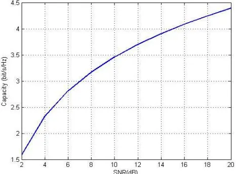
Where h is the normalized complex gain of a fixed wireless channel and is the SNR the plot between the C and SNR will be

Fig 5 Graph Between Capacity And SNR(SISO)

3.2 Multiple Inputs Single Output (MISO)—Transmit diversity

It’s a system with Multiple-antenna arrays are known to

perform better than their single-antenna counterparts, because they can more effectively counter the effects of multipath fading and interference. However, the enhanced performance depends on the amount of channel information at the transmitter and on whether the transmitter is able to take advantage of this information. [2] We have a multiple input–

single-output (MISO) system with N TX antennas and the capacity is given by [9]

C= (1+ / ∑ |ℎ| ) b/sHz ...(2)

Where the normalization by N ensures a fixed total transmitter power and show the absence of array gain in that case.

3.4 Multiple Inputs Multiple Outputs (MIMO)— Transmit-receive diversity

Multiple antennas can be used either at the transmitter or receiver or at both. These various configurations are referred to as multiple input single output MISO, Single Input Multiple Output SIMO, or Multiple Input Multiple Output MIMO. The SIMO and MISO architectures are a form of receive and transmit diversity schemes respectively. On the other hand, MIMO architectures can be used for combined transmit and receive diversity, as well as for the parallel transmission of data or spatial multiplexing. When used for spatial multiplexing MIMO technology promises high bit rates in a narrow band-width and as such it is of high significance to spectrum

[18].

Fig.7 Evolution Of Antenna

4

M

Consider a wireless communication system with Nt transmit (TX) and Nr receive (RX) antennas. The idea is to transmit different streams of data on the different transmit antennas, but at the same carrier frequency. The stream on the p-th transmit antenna, as function of the time t, will be denoted by sp(t). When a transmission occurs, the transmitted signal from the p-th TX antenna might find different paths to arrive at the q-th RX antenna, namely, a direct path and indirect paths through a number of reflections[3]. This principle is called multipath. Suppose that the bandwidth B of the system is chosen such that the time delay between the first and last arriving path at the receiver is considerably smaller than 1/B, then the system is called a narrowband system. For such a system, all the multi-path components between the p-th TX and q-th RX antenna can be summed up to one term, say hqp(t). Since the signals from all transmit antennas are sent at the same frequency, the q-th receive antenna will not only receive signals from q-the p-th, but from all Nt transmitters. This can be denoted by the following equation (the additive noise at the receiver is

SI S

SI S

MI

SO SI

M MI

M

SI S

MISO _SIMO MIM

O Intelligent Antenna

(IA-MIMO)

Network

(Net-MIMO) Multiuser (MU-MIMO) Routing

Mobile Cooperati

Geometr

DPC/BF

MLD

Cellular

MISO

omitted for clarity).

( ) =∑ ℎ ( ) ( ), ...(3 )

To capture all Nt received signals into one equation, the matrix notation can be used:

x(t) = H(t)s(t), ...(4)

where, s(t) is an Nt-dimensional column vector with sp(t) being its p-th element, x(t) is Nr-dimensional with xq(t) on its q-th position and q-the matrix H(t) is Nr × Nt with hqp(t) as its (q,p)-th element, with p = 1, …, Nt and q = 1, …, Nr. A schematic representation of a MIMO communication scheme can be found in Figure 9. Mathematically, a MIMO transmission can be seen as a set of equations (the recordings on each RX antenna) with a number of unknowns (the transmitted signals). If every equation represents a unique combination of the unknown variables and the number of equations is equal to the number of unknowns, then there exists a unique solution to the problem. If the number of equations is larger than the number of unknowns, a solution can be found by performing a projection using the least squares method , also known as the Zero Forcing (ZF) method. For the symmetric case, the ZF solution results in the unique solution.

Fig. 8 Schematic Representation Of A MIMO Communication System.

4.1 Information Theoretic MIMO Capacity

Since feedback is an important component of wireless design (although not a necessary one), it is useful to generalize the capacity discussion to cases that can encompass transmitters having some prior knowledge of channel. To this end, we now define some central concepts, beginning with the MIMO signal model.

r = Hs+n ...(5) In (5), r is the Mx1 received signal vector, s is the Nx1

transmitted signal vector and n is an Mx1 vector of additive noise terms, assumed i.i.d. complex Gaussian with each element having a variance equal to σ . For convenience we

normalize the noise power so that σ = 1 in the remainder of

this section. Note that the system equation represents a single MIMO user communicating over a fading channel with additive white Gaussian noise (AWGN). The only interference present is self-interference between the input streams to the MIMO system. Some authors have considered more general systems but most information theoretic results can be discussed in this simple context, so we use (figure 5) as the basic system equation. Let Q denote the covariance matrix, then the capacity of the system described by (5) is given by [10], [11]

C = [det ( +HQ ∗_{)] b/s/Hz ...(6)}

Here, Q=( ) .

5

H

?

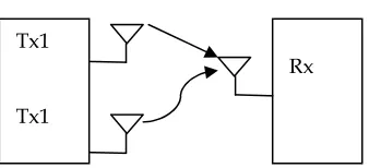
MIMO and “smart antenna” systems may look the same on first examination: Both employ multiple antennas spaced as far apart as practical. But MIMO and smart antenna systems are fundamentally different. Smart antennas enhance conventional, one-dimensional radio systems. The most common smart antenna systems use beam-forming (Fig. 9) or transmit diversity to concentrate the signal energy on the main path and receive combining (Fig. 10) to capture the strongest signal at any given moment.

Fig. 9 Beam-forming (beam steering) employs two transmit antennas to deliver the best multipath signal

Fig. 10 Diversity (receive combining) uses two receive antennas to capture the best multipath signal

Note that beam-forming and receive combining are only multipath mitigation techniques, and do not multiply data throughput over the wireless channel. Both have demonstrated an ability to improve performance incrementally in point-to-point applications (Fig.12) (e.g., outdoor wireless backhaul applications).

RX1

RX2

RX TX1

TX2

TX

H

Tx1

Tx1

Rx

Tx Rx1

95 Fig. 11 Physical resemblance between radio systems using a

combination of beam steering and diversity and MIMO systems

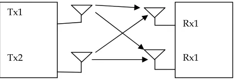
However, while beam-forming and receive combining are valuable enhancements to conventional radio systems, MIMO (Fig.11) is a paradigm shift, dramatically changing perceptions of and responses to multipath propagation. While receive combining and beam-forming increase spectral efficiency one or two b/s/Hz at a time, MIMO multiplies the b/s/Hz.

Fig. 12 MIMO uses multiple transmitters, receivers and antennas to send multiple signals over the same channel, multiplying spectral efficiency.

The powerful effect of smart antenna is that, in the presence of random fading caused by multipath propagation, the probability of losing the signal vanishes exponentially with the number of décor-related antenna elements being used. Clearly, in a MIMO link, the benefits of Conventional smart antennas are retained since the optimization of the multi antenna signals is carried out in a larger space, thus providing additional degrees of freedom. In particular, MIMO systems can provide a joint transmit-receive diversity gain, as well as an array gain upon coherent combining of the antenna elements (assuming prior channel estimation). The underlying mathematical nature of MIMO, where data is transmitted over a matrix rather than a vector channel, creates new and enormous opportunities beyond just the added diversity or array gain benefits- the spectrum efficiency.

6.

S

6.1 Space Time Block Code

When the number of antennas is fixed, the decoding complexity of space–time trellis coding (measured by the

number of trellis states at the decoder) increases exponentially as a function of the diversity level and transmission rate [13]. In addressing the issue of decoding complexity, Alamouti [14] discovered a remarkable space–time block coding scheme for

transmission with two antennas. This scheme supports maximum-likelihood (ML) detection based only on linear processing at the receiver. The very simple structure and linear processing of the Alamouti construction makes it a very attractive scheme that is currently part of both the W-CDMA and CDMA-2000 standards. This scheme was later generalized in [14] to an arbitrary number of antennas. Here, we will briefly review the basics of STBCs. Fig. 6.1.1 shows the baseband representation for Alamouti STBC with two antennas at the transmitter. The input symbols to the space–

time block encoder are divided into groups of two symbols each. At a given symbol period, the two symbols in each group{c , c }are transmitted simultaneously from the two

antennas. The signal transmitted from antenna 1 is c and the

signal transmitted from antenna 2 is c . In the next symbol

period, the signal -c∗ is transmitted from antenna 1 and the

signal c is transmitted from antenna 2. Let h and h be the channels from the first and second TX antennas to the RX antenna, respectively. The major assumption here is that they are scalar and constant over two consecutive symbol periods, that is

ℎ(2nT)≈ℎ(2n+1)T) , I = 1,2

We assume a receiver with a single RX antenna. we also denote the received signal over two consecutive symbol periods as r and r . The received signals can be expressed

as

= ℎ +ℎ + ...(7)

= -ℎ ∗+ℎ ∗+ ...(8)

Where, n and n represent the AWGN and are modeled as

i.i.d. complex Gaussian random variables with zero mean and power spectral density N /2 per dimension. We define the

received signal vector r = [r , r∗] , the code symbol vector

and the noise vector n=[n n∗] . Equations (7) and (8) can be

rewritten in a matrix form as

r=H.c + n ...(9) Where the channel matrix H is defined as

H =

ℎ

ℎ

ℎ

∗

−ℎ

∗

...(10)

H is now only a virtual MIMO matrix with space (columns) and time (rows) dimensions, not to be confused with the purely spatial MIMO channel matrix. The vector is a complex Gaussian random vector with zero mean and covarianceN .I .

Let us define C as the set of all possible symbol pairs c = {c , c }. Assuming that all symbol pairs are equi-probable, and

since the noise vector is assumed to be a multivariate AWGN, we can easily see that the optimum ML decoder is

̌

= arg min ∈ (‖ − . ̃‖ ) ...(11)

The ML decoding rule in (11) can be further simplified by realizing that the channel matrix H is always orthogonal Tx1

Tx2

Rx1

Rx1

Transmitt er

regardless of the channel coefficients. Hence,H∗H =

α. I where α= |h _{| + |}h | . Consider the modified signal

vector given by

̃ = ∗. = . + ...(12)

Where ,n = H∗. n

In this case, the decoding rule becomes

̌ = arg min ∈ (‖ ̃ − . ̃‖ ) ...(13)

Fig.13 Transmit diversity with space time block coding 6.2 Spatial multiplexing

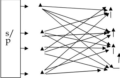
Spatial multiplexing (seen abbreviated SM or SMX) is a transmission technique in MIMO wireless communication to transmit independent and separately encoded data signals, so-called streams, from each of the multiple transmits antennas. Therefore, the space dimension is reused, or multiplexed, more than one time.

If the transmitter is equipped with Nt antennas and the receiver has Nr antennas, the maximum spatial multiplexing order (the number of streams) is

= ( , )

If a linear receiver is used. This means that Ns streams can be transmitted in parallel, ideally leading to an Ns increase of the spectral efficiency (the number of bits per second and per Hz that can be transmitted over the wireless channel). The practical multiplexing gain can be limited by spatial correlation, which means that some of the parallel streams may have very weak channel gains. The spatial multiplexing(SM) delivers parallel streams of data by exploiting multipath. It can double (2x2) or quadruple (4x4) capacity and throughout. It gives higher capacity where RF conditions are favorable and the users are closer to the BTS. In spatial multiplexing, different information is transmitted simultaneously over N transmit antennas increasing the data rate at short distance and providing high spectral efficiency similar to increasing the constellation size, but without suffering from a power penalty. The spatial multiplexing is sometime also referred as direct

transmission or simply MIMO. The receiver has to decouple the N spatial streams to recover the transmitted information. Optimal detection tends to be complex and several suboptimal low-complexity detectors have been devised, ranging from the simple zero forcing to complex soft a posteriori probability detection. An example of spatial multiplexing is shown in a figure 14,which improves the average capacity behavior by sending as many independent signals as we have antennas for a specific error rate In the uplink scenario, a base station employs multiple receive antennas and beam forming to separate transmissions from the different mobiles. More recently, transmit beam forming/pre-coding for multi user downlink transmission is drawing increasing attention.

S1

Fig.14 Example of Spatial Multiplexing

Layered space-time architectures exploit the spatial multiplexing gain by sending independently encoded data streams in diagonal layers(D-BLAST) as originally proposed or in horizontal layers, which is the so-called vertical layered space-time(V-BLAST) scheme, depicted in fig 16, originally invented by Bell labs.[15].the receiver must de-multiplex the spatial channels in order to detect the transmitted symbols. Various estimation and zero-forcing, which use simple matrix inversion but give poor results when the channel matrix is ill conditioned, minimum mean square error(MMSE), more robust in that sense but provides limited enhancement if knowledge of the noise/interference is not used, and maximum likelihood(ML), which is optimal in the sense that it compares all possible combinations of symbols but can be too complex, especially for high-order modulation.

6.2.1 D-Blast

In wireless systems, radio waves do not propagate simply from transmit antenna to receive antenna, but bounce and scatter randomly off objects in environment. This scattering is known as multipath as it result in multiple copies of the transmitted signals arriving at the receiver via different scattered paths. Multipath has always been regarded as impairment, because the images arrive at the receiver at slightly different times and thus can interfere destructively, canceling each other out. However recent advances in information theory have shown that, with simulations use of antenna arrays at both base station and terminal, multipath interference can be not only mitigated, but actually exploited to establish multiple parallel Info

rma ti-on

Constel lation mapper

ST Block Code [ S ]

s/

97 channels that operate simultaneously and in the same

frequency band. Based on this fundamental idea, a class of layered space-time architecture was proposed and labeled BLAST. Using BLAST the scattering characteristics of the propagation environment is used to enhance the transmission accuracy by treating the multiplicity of the propagation environment is used to enhance the transmission accuracy by treating the multiplicity of scattering paths as separate parallel sub channels. The original scheme D-BLAST was a wireless set up that used a multi element antenna array at both the transmitter and receiver, as well as diagonally layered coding sequence. The coding sequence was to be dispersed across diagonals in space-time. In an independent Rayleigh scattering environment, this processing structure leads to theoretical rates that grow linearly with the number of antennas these rates approaching 90% of Shanon capacity. Rayleigh scattering of light off the molecules of air, and can be extended to scattering from particles up to about a tenth of the wavelength of light. Rayleigh scattering can be considered to be elastic scattering because the energies of scattered photons do not change.

Antenna index

Time Fig.15 D-BLAST

6.2.2 V-Blast

The Vertical BLAST or V-BLAST architecture [3] is a simplified version of D-BLAST that tries to reduce its computational complexity. We use space time block code in V-BLAST and it can be decoded by ML.

A 1

A 1

A 1

A 1

…………

………

demodul

ated

demod

_ulated

A

_A

2

₂

A

3

A

3

A

4

A

3

…………

………..

demod

ulated

demod

ulated

A

4

A

3

A

4

A

4

…………

……….

demod

ulated

demod

ulated

Fig.16 V-Blast Architecture

7

C

an equivalent SISO system while maintaining the same bandwidth and power.

7.1. Capacity Enhancement Using MIMO

For a memory less 1x1 (SISO) system the capacity is given by:

C= (1+ |ℎ| ) b/s/Hz ...(14)

Where h is the normalizes complex gain of a fixed wireless channel or that of a particular realization of a random channel. As we deploy more RX antennas the statistics of capacity will improve and with M RX antennas, we have a SIMO system with capacity given by

C= (1+ ∑ |ℎ| ) b/sHz ...(15)

Where h is the gain of RX antenna. Note that the crucial

feature of (15) is that increasing the value of M only result in a logarithmic increase in average capacity. Similarly, if we opt for transmit diversity, in the common case, where the transmit does not have channel knowledge, we have a multiple input–

single-output (MISO) system with N TX antennas and the capacity is given by [9]

C= (1+ / ∑ |ℎ| ) b/sHz ...(16)

Where the normalization by N ensures a fixed total transmitter power and shows the absence of array gain in that case (compared to the case in (15), where the channel energy can be combined coherently). Again, note that capacity has a logarithmic relationship with N. Now, we consider the use of diversity at both transmitter and receiver giving rise to a MIMO system. For N TX and M RX antennas, we have the now famous capacity equation [9], [10], [11]

C= [det( +( / )H ∗)]

...(17)

Where ( * ) means transpose-conjugate and H is the MxN channel matrix. Note that both (16) and (17) are based on equal power (EP) uncorrelated sources, hence, the subscript in (4). Foschini [9] and Telatar [10] both demonstrated that the capacity in (17) grows linearly with m=min(M,N) rather than logarithmically [as in (17)]. This result can be intuited as follows: the determinant operator yields a product of m=min(M,N) nonzero Eigen values of its (channel-dependent) matrix argument, each Eigen value characterizing the SNR over a so-called channel Eigen mode. An Eigen mode corresponds to the transmission using a pair of right and left singular vectors of the channel matrix as transmit antenna and receive antenna weights, respectively. Thanks to the properties of the MIMO, the overall capacity is the sum of

capacities of each of these modes, hence the effect is capacity multiplication. Clearly, this growth is dependent on properties of the Eigen values. If they decayed away rapidly then linear growth would not occur. However (for simple channels), the Eigen values have a known limiting distribution [12] and tend to be spaced out along the range of this distribution. Hence, it is unlikely that most Eigen values are very small and the linear growth is indeed achieved. For the i.i.d. Rayleigh fading case we have the impressive linear capacity growth discussed above. For a wider range of channel models including, for example, correlated fading and specular components, we must ask whether this behavior still holds. Below we report a variety of work on the effects of feedback and different channel models. It is important to note that (17) can be rewritten as [10].

C=∑ log (1+( ρ/N)λ) ...(18)

min(M,N), and

W= HH∗, M≤N

H∗H, N < ...(19)

This formulation can be easily obtained from the direct use of Eigen value properties. Alternatively, we can decompose the MIMO channel into m equivalent parallel SISO channels by performing singular value decomposition (SVD) of [3], [21].

7.2 Capacity of MIMO

Fig. 18 Capacity Enhancement in MIMO

8.

C

This report reviews the major features of MIMO links for use in future wireless networks. Information theory reveals the great capacity gains which can be realized from MIMO. Whether we achieve this fully or at least partially in practice depends on a sensible design of transmit and receive signal processing algorithms. It is clear that the success of MIMO algorithm integration into commercial standards such as 3G, WLAN, and beyond will rely on a fine compromise between rate maximization (BLAST type) and diversity (spa

solutions, also including the ability to adapt to the time changing nature of the wireless channel using some form of (at least partial) feedback. To this end more progress in modelling, not only the MIMO channel but its specific dynamics, will be required. As new and more specific channel models are being proposed it will useful to see how those can affect the performance tradeoffs between existing transmission algorithms and whether new algorithms, tailored to specific models, can be developed. Finally, upcoming trials and performance measurements in specific deployment conditions will be key to evaluate precisely the overall benefits of MIMO systems in real-world wireless scenarios such as UMTS.

Acknowledgment

The authors would like to thank Mr. Akhileshwar Sharma, Ms. Elena Malova &Mr. H.S Rai from the Dept. Of Electronics Design & Technology of National Institute Of Electronics & Information Technology Gorakhpur for his insightful feedback and commentary about their full support in res

Capacity Enhancement in MIMO

the major features of MIMO links for use in future wireless networks. Information theory reveals the great capacity gains which can be realized from MIMO. Whether we achieve this fully or at least partially in practice depends on a of transmit and receive signal processing algorithms. It is clear that the success of MIMO algorithm into commercial standards such as 3G, WLAN, and beyond will rely on a fine compromise between rate maximization (BLAST type) and diversity (space–time coding)

solutions, also including the ability to adapt to the time changing nature of the wireless channel using some form of (at least partial) feedback. To this end more progress in modelling, not only the MIMO channel but its specific will be required. As new and more specific channel models are being proposed it will useful to see how those can affect the performance tradeoffs between existing transmission algorithms and whether new algorithms, tailored to specific oped. Finally, upcoming trials and performance measurements in specific deployment conditions will be key to evaluate precisely the overall benefits of MIMO

world wireless scenarios such as UMTS.

thank Mr. Akhileshwar Sharma, Ms. Elena Malova &Mr. H.S Rai from the Dept. Of Electronics Design & Technology of National Institute Of Electronics & Information Technology Gorakhpur for his insightful feedback and commentary about their full support in research work.

References

[1] A. Goldsmith et al., “Capacity Limits of MIMO Channels,”

IEEE JSAC, vol. 21, June 2003, pp. 684

[2] H. Weingarten, Y. Steinberg, and S. Shamai, “The Capacity Region of the Gaussian MIMO Broadcast Channel,” Proc. Conf. Info. Sciences and Systems (CISS),

Princeton, NJ, Mar. 2004.

[3] D. Gesbert, M. Shafi, D. S. Shiu, P. Smith, and A. Naguib,

“From theory to practice: An overview of MIMO space coded wireless systems,”

IEEE J. Select. Areas Commun. Special Issue on MI Systems, pt. I,vol. 21, pp. 281–

[4] T. Svantesson and A. L. Swindlehurst, “A Performance Bound for Prediction of a Multipath MIMO Channel,” Proc. 37th Asilomar Conf. Sig., Sys., and Comp., Session: Array Processing for Wireless Commun., Pa

Nov. 2003.

[5] Siavash M. Alamouti “A Simple Transmit Diversity Technique for Wireless Communications”, IEEE JSAC, vol. 16, no. 8, October 1998, pp. 1452

[6] Siavash M. Alamouti “A Simple Transmit Diversity Technique for Wireless Communications”, IEEE JSAC, vol. 16, no. 8, October 1998, pp. 1456.

[7] Vahid Tarokh “Space–Time Codes for High Data Rate

Wireless Communication: Performance Criterion and Code Construction”, IEEE Transactions on Information Theory, vol. 44, no. 2, March 1998, p. 746.

[8] “A new bandwidth efficient transmit antenna modulation diversity scheme for linear digital modulation,” in Proc. IEEE’ICC, 1993, pp. 1630–1634.

[9] G. J. Foschini and M. J. Gan

communications in a fading environment when using multiple antennas,” Wireless Pers. Commun., vol. 6, pp. 311–335, Mar. 1998

[10] E. Telatar, “Capacity of multiantenna Gaussian channels,” AT&T Bell Laboratories, Tech. Memo., June 1995

[11] I. E. Telatar, “Capacity of multi antenna Gaussian channels,” Eur. Trans. Commun., vol. 10, no. 6, pp. 585 595, 1999.

[12] J. W. Silverstein, “Strong convergence of the empirical distribution of eigenvalues of large dimensional random matrices,” J. Multivariate Anal., vol. 55, no. 2, pp. 331

339, 1995.

[13] V. Tarokh, N. Seshadri, and A. R. Calderbank, “Space time codes for high data rate wireless communication: Performance criterion and code construction,” IEEE Trans. Inform. Theory, vol. 44, pp. 744

[14] S. Alamouti, “Space block coding: A simple transmitter diversity technique for wireless communications,” IEEE J. Select. Areas. Commun., vol. 16, pp. 1451

1998.

[15] Bell Laboratories Layered Space

J. Foschini (1996) A. Hottinen, O. Tirkkonen, and R. Wichman, Multi-antenna transceiver

[16] Techniques for 3G and beyond. John Wiley and Sons, January 2003.

[17] Wireless Communication by Theodore S.Rappaport. 99 A. Goldsmith et al., “Capacity Limits of MIMO Channels,”

IEEE JSAC, vol. 21, June 2003, pp. 684–702.

H. Weingarten, Y. Steinberg, and S. Shamai, “The Capacity Region of the Gaussian MIMO Broadcast nf. Info. Sciences and Systems (CISS), D. Gesbert, M. Shafi, D. S. Shiu, P. Smith, and A. Naguib,

“From theory to practice: An overview of MIMO space-time

IEEE J. Select. Areas Commun. Special Issue on MIMO

–302, Apr. 2003.

T. Svantesson and A. L. Swindlehurst, “A Performance Bound for Prediction of a Multipath MIMO Channel,” Proc. 37th Asilomar Conf. Sig., Sys., and Comp., Session: Array Processing for Wireless Commun., Pacific Grove, CA, Siavash M. Alamouti “A Simple Transmit Diversity Technique for Wireless Communications”, IEEE JSAC, vol. 16, no. 8, October 1998, pp. 1452-1455.

Siavash M. Alamouti “A Simple Transmit Diversity Technique for Wireless Communications”, IEEE JSAC, vol. 16, no. 8, October 1998, pp. 1456.

Time Codes for High Data Rate Wireless Communication: Performance Criterion and on”, IEEE Transactions on Information Theory, vol. 44, no. 2, March 1998, p. 746.

“A new bandwidth efficient transmit antenna modulation diversity scheme for linear digital modulation,” in Proc.

1634.

G. J. Foschini and M. J. Gans, “On limits of wireless communications in a fading environment when using multiple antennas,” Wireless Pers. Commun., vol. 6, pp. E. Telatar, “Capacity of multiantenna Gaussian channels,” AT&T Bell Laboratories, Tech. Memo., June I. E. Telatar, “Capacity of multi antenna Gaussian channels,” Eur. Trans. Commun., vol. 10, no. 6, pp. 585–

J. W. Silverstein, “Strong convergence of the empirical distribution of eigenvalues of large dimensional random ariate Anal., vol. 55, no. 2, pp. 331–

V. Tarokh, N. Seshadri, and A. R. Calderbank, “Space–

time codes for high data rate wireless communication: Performance criterion and code construction,” IEEE Trans. Inform. Theory, vol. 44, pp. 744–765, Mar. 1998.

S. Alamouti, “Space block coding: A simple transmitter diversity technique for wireless communications,” IEEE J. Commun., vol. 16, pp. 1451–1458, Oct.

Bell Laboratories Layered Space-Time (BLAST), Gerard. ) A. Hottinen, O. Tirkkonen, and R. antenna transceiver

[18] Wikipedia

[19] Markku Juntti, et. al. ,”MIMO Communications with Applications to 3G and 4G”, Oulu University,

[20] Aalborg University, Lecture notes, URL: http://kom.aau.dk/~imr/RadioCommIII

[21] Royal institute of technology, stockholm, lecture notes, url: