Multi-Robot Active Information Gathering Using Random Finite Sets

(1)

University of Pennsylvania

ScholarlyCommons

Publicly Accessible Penn Dissertations

1-1-2015

Multi-Robot Active Information Gathering Using

Random Finite Sets

Philip Dames

University of Pennsylvania, [email protected]

Follow this and additional works at:

http://repository.upenn.edu/edissertations

Part of the

Computer Sciences Commons,

Mechanical Engineering Commons, and the

Robotics

Commons

This paper is posted at ScholarlyCommons.http://repository.upenn.edu/edissertations/1676

Recommended Citation

Dames, Philip, "Multi-Robot Active Information Gathering Using Random Finite Sets" (2015).Publicly Accessible Penn Dissertations. 1676.

(2)

Multi-Robot Active Information Gathering Using Random Finite Sets

Abstract

Many tasks in the modern world involve collecting information, such as infrastructure inspection, security and surveillance, environmental monitoring, and search and rescue. All of these tasks involve searching an

environment to detect, localize, and track objects of interest, such as damage to roadways, suspicious packages, plant species, or victims of a natural disaster. In any of these tasks the number of objects of interest is often not known at the onset of exploration. Teams of robots can automate these often dull, dirty, or dangerous tasks to decrease costs and improve speed and safety. This dissertation addresses the problem of automating data collection processes, so that a team of mobile sensor platforms is able to explore an environment to determine the number of objects of interest and their locations. In real-world scenarios, robots may fail to detect objects within the field of view, receive false positive measurements to clutter objects, and be unable to disambiguate true objects. This makes data association, i.e., matching individual measurements to targets, difficult. To account for this, we utilize filtering algorithms based on random finite sets to simultaneously estimate the number of objects and their locations within the environment without the need to explicitly consider data association. Using the resulting estimates they receive, robots choose actions that maximize the mutual information between the set of targets and the binary events of receiving no detections. This effectively hedges against uninformative actions and leads to a closed form equation to compute mutual information, allowing the robot team to plan over a long time horizon. The robots either communicate with a central agent, which performs the estimation and control computations, or act in a decentralized manner. Our extensive hardware and simulated experiments validate the unified estimation and control framework, using robots with a wide variety of mobility and sensing capabilities to showcase the broad applicability of the framework.

Degree Type Dissertation

Degree Name

Doctor of Philosophy (PhD)

Graduate Group

Mechanical Engineering & Applied Mechanics

First Advisor Vijay Kumar

Subject Categories

(3)

MULTI-ROBOT ACTIVE INFORMATION GATHERING USING RANDOM FINITE SETS

Philip M. Dames A DISSERTATION

in

Mechanical Engineering and Applied Mechanics Presented to the Faculties of the University of Pennsylvania

in

Partial Fulllment of the Requirements for the Degree of Doctor of Philosophy

2015

Vijay Kumar, Supervisor of Dissertation

UPS Foundation Professor of Mechanical Engineering and Applied Mechanics

Prashant Purohit, Graduate Group Chairperson

Associate Professor of Mechanical Engineering and Applied Mechanics

Dissertation Committee

George Pappas, Professor of Electrical and Systems Engineering

(4)

c

COPYRIGHT

2015

(5)

(6)

Acknowledgments

I would like to thank my advisor, Vijay Kumar, whose has guided and supported me over the last ve years. I sincerely appreciate all of the opportunities that he has provided for me to become an independent scholar, to meet interesting people, and to travel across the globe. I would also like to thank the rest of my dissertation committee, George Pappas, Dan Koditschek, and Mac Schwager, for taking the time to serve on my committee and for the interesting discussions over the past several years. Mac Schwager, in particular, helped me build a solid foundation for my research during his tenure as a postdoctoral fellow as Penn. Kevin Lynch, Paul Umbanhowar, and Tom Vose rst got me interested in the eld of robotics through their mentorship during my undergraduate years. They really challenged me to do independent work and gave me a head start for when I arrived at Penn.

I would like to thank all of the current and former members of GRASP that I have had the pleasure to work with. In particular I would like to thank Ben Charrow for helping turn a mechanical engineer into a passable computer scientist and for the many long discussions about probability, information theory, and life. I would also like to thank Justin Thomas for helping me nally learn how to use quadrotors during the last month of my dissertation. I would never have gotten here without the constant support from my family. My parents provided me with every opportunity to succeed in life and I can't thank them enough.

(7)

ABSTRACT

Philip M. Dames Vijay Kumar

(8)

List of Tables

1 Example information gathering applications. . . 2

2 Table of symbols. . . 33

3 Comparison of approximation methods for uniform belief. . . 54

(12)

List of Figures

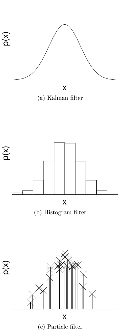
1 Example unimodal distribution represented by (a) a Gaussian distribution, (b)

a histogram lter, and (c) a particle lter. . . 9

2 Examples of random nite sets with 0 to 3 elements drawn from the square environment. . . 19

3 Illustration of our multi-robot multi-target localization algorithm. . . 35

4 An simple example showing the cell renement and merging procedures. . . 45

5 In this situation the team of robots, with the footprints of the individual robots shown by the circles, is divided into two cliques C1 ={1,2,4}, C2={3}. . . 49

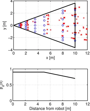
6 The locations of the robots in the test environment. . . 53

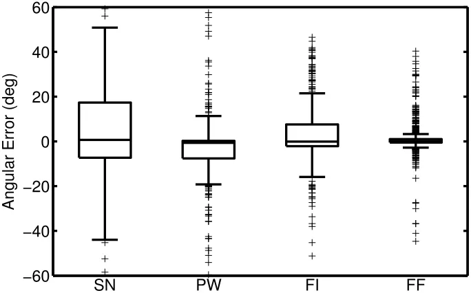
7 Box plots showing the error in angle of the gradient approximations for each of the approximation methods, measured in degrees. . . 55

8 Simulation results in the trial environment. . . 57

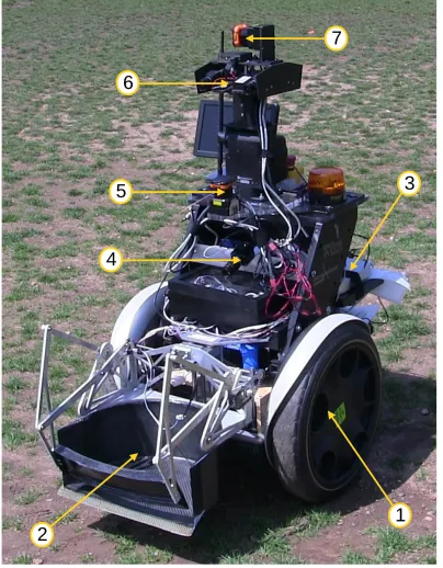
9 Robot platform. . . 59

10 Experimental detection model. . . 60

11 Cell-based measurement model. . . 61

12 Experimental results showing the true and estimated object positions as mea-sured in the body frame of the robot. . . 63

13 Sample results from experimental data with a single target. . . 65

14 Sample results from experimental data with two targets. . . 67

15 Experimentally determined MAD sensor detection models used for target de-tection and localization. . . 69

16 Experimental results for single robot experiments. . . 70

17 Localization results for a single real-world quadrotor. The orange diamonds indicate the true target positions and shading within each cell is the probability of occupancy. . . 71

18 Box plots of the time to completion for the simulated and hardware MAD experiments. . . 71

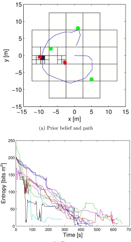
19 Simulation results for two robot experiments. (a) The time evolution of the target entropy. (b) The time evolution of the expected number of targets. . . . 73

20 Diagram of the decentralized network structure. . . 75

21 Example action sets for a robot in free and cluttered space over multiple length scales. . . 80

22 Finite state machine of the three control modes. . . 84

(13)

24 Detection model used in simulations. . . 93 25 Expected cardinality and nal PHD for PHD and CPHD lters with innite

and nite sensor eld of view. . . 94 26 Expected cardinality and nal PHD in two simulated environments. . . 96 27 Data showing the performance with very large numbers of targets in

environ-ment 3. . . 97 28 Example environment used for simulations with decentralized implementation. . 99 29 Time evolution of the entropy of the target RFS for a variety of team sizes and

footprint radii. . . 100 30 Time spent in each control mode, Exploit, Check-in, and Explore. . . 102 31 Plots showing the time evolution of the number of true targets and false targets.102 32 A Scarab robot with two targets in the experimental environment. . . 103 33 A oorplan of the Levine environment used in the hardware experiments. . . . 104 34 A pictogram of the laser detection model, wheredtis the diameter of the target,

θsep is the angular separation between beams, and r is the range. . . 106 35 A pictogram of the clutter model, where θc is the width of the clutter peaks

centered at±π

2, and the bearing falls within the range [− 3π

4 , 3π

4 ]. . . 107 36 Plots of the performance of a team of three real-world robots exploring the

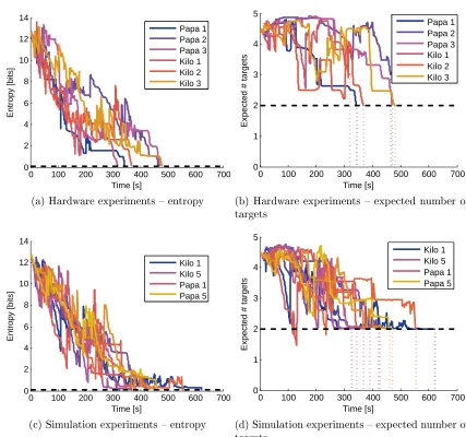
Levine environment using planning mode 1. . . 110 37 Plots of the performance for teams of 1, 3, and 5 real-world robots exploring

the Levine environment using planning mode 3. . . 111 38 Plots of the performance for teams of three real and simulated robots exploring

the Levine environment using planing mode 1. . . 113 39 Plots of the performance for a team of three simulated robots exploring the

Levine environment using planning modes 15. . . 114 40 Plots of the performance for a team of three simulated robots exploring the

Levine environment for 1, 15, or 100 targets using planning mode 2. . . 116 41 Plots of the performance for a team of three simulated robots exploring a second

environment using planning mode 2. . . 118 42 Plots of the performance for a team of three simulated robots equipped with

range-only sensors exploring the Levine environment using planning mode 2. . . 120

43 The mean and covariance of the Gaussian Process regression motion model over a patch of the environment. . . 129 44 (a) The area of interest, a roughly 6.15×5.56km region surrounding downtown

San Francisco. (b) The probability of target survival as a function of position. . 130 45 Empirical target birth PHD. . . 131 46 Sample trajectories. . . 135 47 Ratio of the expected number to the true number of targets over a single run

for R= 2 andT = 6. . . 137 48 The elevation of the robots over a single run for R= 2 andT = 6. . . 138 49 The entropy of the target set over a single run for R= 2 andT = 6. . . 139 50 Average ratio of the expected number of targets to the true number of targets

over a single run. . . 141 51 Average fraction of the number of true targets within the team's eld of view

(14)

52 Average ratio of the expected number of targets to the true number of targets

within the team's eld of view over a single run. . . 143

53 Average elevation of the robots over a single run. . . 144

54 Average entropy of the target set over a single run. . . 145

55 Performance of our framework with static targets. . . 146

56 Photo of an Ascending Technology Hummingbird MAV hovering over a mag-netic target. A second target may be seen in the background. . . 154

57 Experimental results of the magnetic eld strength as a function of the 2D position of the MAVs in the baseline training runs. . . 155

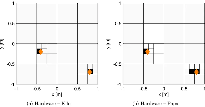
58 Experimental results of the deviation of the magnetic eld due to the addition of a magnet as a function of the true distance to the magnet for (a) MAV Kilo and (b) MAV Papa. . . 156

59 Experimental MAD sensor detection models. . . 157

60 A Scarab robot with two targets in the experimental environment. . . 159

61 A oorplan of the environment used in the hardware experiments. Dierent starting locations for the robots are labeled in the map. . . 159

62 Example action set with a horizon of T = 3steps and three length scales. Each action is a sequence of T poses at which the robot will take a measurement, denoted by the hollow circles. . . 161

63 An example laser scan from the oce environment. . . 161

64 A pictogram and experimental best t of the laser detection model. . . 162

65 Detection model sum of squares error (SSE) (blue circles) and the fraction of measurements that were classied as detections (orange exes) as a function of the measurement noise parameter. . . 164

66 A pictogram and experimental best t of the clutter model. . . 165

(15)

Chapter 1 Introduction

Mobile computers, sensors, and robot platforms are becoming more powerful and less expen-sive, particularly as smartphones, wearable devices, and hobby robots become mainstream. These technologies can be combined to create low cost mobile sensor platforms. While in-dividual robots built from low-cost components have limited capabilities, putting multiple robots together into a team increases their collective computational power, the eective sen-sor eld of view, and the robustness of the team to individual agent or sensen-sor failure. As the technologies continue to mature, teams of robots will automate more tasks that are dull, dirty, dangerous, or not possible for humans to perform.

(16)

Table 1: Example information gathering applications.

Scenario Targets Number of targets? Targets moving?

Infrastructure inspection Damage or wear Small No

Security and surveillance Intruders Small Sometimes

Map registration Smart devices Large No

Precision agriculture Crop health Large No

Environmental monitoring Plant species Large Sometimes

Reconnaissance Enemy assets Large Sometimes

Search and rescue People Large Sometimes

to build a map; and search and rescue, where the robots seek out lost or injured individuals. Such tasks span many geographic and temporal scales: search and rescue missions are often conned to a small area and must be completed in a manner of minutes while environmental monitoring missions may take place over many kilometers and last months or years. Table 1 details these information gathering scenarios.

All of these tasks share the same high-level goal: to identify the locations of all of the objects of interest e.g., intruders or map landmarks, within the environment. However, the number of objects of interest is often not known at the onset of exploration, and the objects may not be uniquely identiable. For example, in an environmental monitoring task two plants of the same species may look identical. Additionally, the sensors on board the robot may be unreliable: failing to detect objects within their eld of view, providing false positive measurements, and providing noisy measurements of true objects. The number of objects within the sensor eld of view may also change over time, due to motion of the robots, motion of the objects, or obstacles in the environment. It is important for any perception and decision making framework to take these uncertainties into account when estimating the state of the surrounding environment and selecting actions to improve this estimate.

(17)

algorithms to account for the uncertainties in the environment and sensor readings. While the former group of estimation algorithms has received some attention from the active sensing community, the latter has not. Chapter 2 provides a survey of tracking algorithms, a brief tutorial on the methods used in this dissertation, and an overview of active sensing methods. This dissertation contributes to these developing technologies by enabling teams of mo-bile robots to autonomously explore and gather information with limited a priori knowledge of the given situation, turning sensor data into actionable information. In any of these in-formation gathering scenarios there may be uncertainty in the environment, the number of objects of interest may be unknown, or there may be unpredictable physical phenomena. This research aims to improve the performance of robotic teams in real-world application domains by building systems that explicitly consider such uncertainties. The closed form control objective developed in this dissertation accounts for these uncertainties while allow-ing a small team of robots to jointly plan actions over a nite horizon in real time. Robots working together as a team are able to gather information more quickly and eciently than robots exploring independently. However, such coordination is not possible in many situ-ations due to limitsitu-ations in wireless communication. The proposed framework is exible, allowing the team the use either a central planner when possible or decentralized coalitions that are formed online when communication is limited.

(18)

to environmental monitoring and surveillance.

(19)

Chapter 2 Background Material

This chapter reviews many of the multi-object estimation and multi-robot control concepts that will be used throughout the dissertation. Section 2.1 reviews concepts in single- and multi-target tracking and justies our selection of tracking algorithms. Section 2.2 provides a tutorial on nite set statistics, the mathematical tool used in our estimation algorithm. Finally, Section 2.3 provides an overview of active information gathering approaches and positions our framework with the current state of scholarship and research on the subject.

2.1 Target Tracking

(20)

This section reviews common methods for Bayesian single-target tracking, namely the Kalman lter, the histogram lter, and the particle lter. We will then discuss existing methods to extend these single-target approaches to situations with multiple targets. Finally we present Bayesian methods for multi-target tracking, focusing on approaches where the number of targets and the data association are both unknown.

2.1.1 Single-Target Tracking

Single-target tracking is a canonical problem in estimation theory and robotics. In the single-target scenario, the data association is known since there is only a single single-target. Thus, the problem is simply how to use the incoming measurements from the sensors to update the belief about the state of the target. LetE be the environment that the robot team explores and letq∈E be the pose of the robot. Let x∈E be the state of the target and let z be a

measurement from a robot's sensor. Since there is uncertainty associated with each of these quantities, we will use a probabilistic representation.

It is possible for some targets to move over time. To account for this possibility, we dene the motion modelf(x|ξ), which denes the probability of a target with initial state

ξ moving to statex. In situations with stationary targets the transition model is simply the

identity map, f(x|ξ) =δξ(x), whereδξ(x)is the Kronecker delta function.

Letg(z|x,q)be the probability of a robot with poseqreceiving a measurementzfrom

a target with statex. Letp(x) be the prior probability that the target has statex. We may

then use Bayes' rule to nd the posterior probability,

p(x|z) = p(x,z) p(z) =

p(z|x)p(x)

R

p(x,z)dx =

g(z|x, q)p(x)

R

g(z|x,q)p(x)dx. (2.1)

(21)

Kalman Filter

The Kalman lter (KF) [53] is an implementation of the Bayes lter for linear Gaussian systems. This means that the target state is represented by a Gaussian distribution, the measurement and motion models are linear, and all noise is additive Gaussian. The Gaussian distribution takes the form

p(x) = det(2πΣ)−1/2exp

−1

2(x−µ)

T_Σ−1

(x−µ)

, (2.2)

whereµis the mean of the distribution,Σis the covariance matrix,det(·)is the determinant of a matrix, and xis a vector of the target state. Figure 1a shows an example distribution.

Note that this distribution is fully characterized by the mean vector and covariance matrix. The Kalman lter provides a set of rules to update these parameters.

Let the transition model be

x_t|t−1 =Atxt−1+bt+t, (2.3)

whereAtis a matrix, xt−1 is the prior state at timet−1,xt|t−1 is the predicted state,btis

an ane term (often representing the control input at timet), and t is a Gaussian random

vector with zero mean and covariance Rt. Then the update equations are

µt|t−1 =Atµt−1+bt (2.4)

Σ_t|t−1 =AtΣt−1ATt +Rt. (2.5)

Let the measurement model be

z=Ctxt+δt, (2.6)

(22)

Then the update equations are

Kt= Σt|t−1CtT(CtΣt|t−1CtT +Qt)−1 (2.7)

µt=µt|t−1+Kt(zt−Ctµt|t−1) (2.8)

Σt= (I−KtCt)Σt|t−1, (2.9)

whereI is the identity matrix andKtis the so-called Kalman gain. Intuitively, the Kalman

gain describes how much to trust the measured versus the predicted target location. The termzt−Ctµt|t−1is known as the innovation of the observation, and represents the dierence between the predicted and actual measurement.

The Kalman lter can be extended to deal with non-linear measurement and motion models by linearizing about the mean, leading to the extended Kalman lter (EKF) [97, Chapter 3.3], or by using the unscented transform, leading to the unscented Kalman lter (UKF) [97, Chapter 3.4].

Histogram Filter

While the Kalman lter is computationally ecient and works well in some scenarios, it has a number of shortcomings. Namely, it can accumulate signicant error when the mea-surement model is highly non-linear. Also the probabilistic representation is inherently unimodal, meaning it cannot be used to represent distributions with multiple, disjoint hy-potheses. In some situations, particularly with non-linear measurements such as range-only measurements, multimodal distributions are common.

(23)

x

p(x)

(a) Kalman lter

x

p(x)

(b) Histogram lter

x

p(x)

(c) Particle lter

(24)

The prediction and update rules are then quite simple,

pk,t|t−1 = X

i

f(xk,t |xi,t−1)pi,t−1 (2.10)

η =X

k

g(zt|xk)pk,t|t−1 (2.11)

pk,t =η−1g(zt|xk)pk,t|t−1 (2.12)

where pk,t is the probability that the target is in region k at time t (i.e., xt ∈xk,t) andη

is a normalization constant. The accuracy and computational complexity of the histogram lter will depend upon the size of the histogram bins.

Particle Filter

The particle lter (PF) [97, Chapter 4.3] provides an alternative to the histogram lter. In this case the arbitrary distribution is represented by a set of weighted particles, rather than a set of cells. These particles may take arbitrary locations, though it is desirable to have more particles in areas with higher likelihood to better capture the behavior of the distribution. Let the number of particles be N, wherexi,t is the ith particle state (i.e., hypothesis) and

wi,tis the weight (i.e., likelihood) of the particle. Figure 1c shows an example set of particles

that approximates the distribution in Figure 1a.

In the most basic implementation of the PF, each particle moves according to the motion model, i.e.,xi,t|t−1∼f(· |xi,t−1). The weight of the particle is then updated

η=X

k

g(zt|xk,t|t−1)wk,t|t−1 (2.13)

wk,t=η−1g(zt|xk,t|t−1)wk,t|t−1. (2.14)

(25)

2.1.2 Multi-Target Tracking

The multi-target tracking problem is more complicated. The simplest case is when the num-ber of targets and the data association are both known. In this case, a separate single-target lter may be used to track the states of the dierent targets xi. Each measurement is then

used to update the associated target estimate. This is an intuitive and appealing approach, and much of the work on multi-target tracking attempts to reformulate the problem as a collection of single-target problems.

Having known data association is equivalent to stating that the sensor is able to uniquely identify individual targets and that it is able to do so without error. This is a valid assump-tion in some settings, e.g., localizing wireless sensors using the MAC address to provide a unique label [12]. However, in many other systems there could easily be errors in the data association, e.g., when tracking people in a crowd using facial recognition software, or association may not be possible, e.g., when mapping a set of identical-looking doors in an oce environment. In these cases, we must solve both the data association and tracking problems.

One common method of multi-target tracking with unknown associations is to use the maximum likelihood association. This has been used successfully in a variety of situations, including simultaneous localization and mapping [31]. In this approach, each measurement is checked against each object. Any measurement that is suciently close to the estimated target state is accepted as an association, ensuring that only one measurement is associated with each object. All other measurements are discarded or are used to initialize new target estimates. While this approach is simple to understand and implement, all of the associations decisions are hard, meaning that there is no notion of uncertainty. This ideas runs counter to the probabilistic approach often used in tracking problems, and means making an incorrect association can have a long-lasting impact on the estimate. Mullane et al. [76] show examples of such errors in the context of feature-based mapping.

(26)

joint target state distribution conditioned on each data association. Let θ : {1, . . . , n} →

{0,1, . . . , m} be an association between a set of n targets and a set of m measurements.

Note that θ(j) = 0 means that the target is not detected, i.e., a false negative, and any element of {1, . . . , m}not in the range of θ({1, . . . , n}) is a false positive. Then the update step, for a given association, becomes

pt(x|z, θ) =η−1g(z|x, θ)pt|t−1(x). (2.15)

However, the number of associations grows combinatorially in the number of targets and measurements, making this approach intractable for large problems or long time horizons. The explosive growth in the number of association histories over time can be reduced, for example, by keeping the N best associations at each time step or the N best association histories. However, this still requires computing all possible associations at each time step. The Probabilistic MHT (PMHT) method [95, Chapter 4.6] relaxes the MHT assumptions to allow for soft associations and to allow more than one measurement to be associated with a single target. It also assumes that the single-target measurement likelihoods are condition-ally independent given a data association. PMHT then uses the expectation maximization (EM) algorithm to nd the maximum a posteriori (MAP) estimate of the targets given the measurements. In this case, the association likelihoods and the number of targets are assumed to be known and xed. PMHT is a batch method, solving for the sequence of maximum likelihood target tracks using a sequence of measurement sets. This makes it unsuitable for real-time applications.

(27)

association. In this approach, we compute the soft association matrix A, with elements

amn = X

θ|θ(m)=n

p(θ|z) (2.16)

and leta¯n= 1−Pmamnbe the probability that no measurement is associated to target n.

Then the update rule for target nJPDA is

pt(xn) = ¯anpt|t−1(xn) + X

m

amnη−1g(zm |xn)pt|t−1(xn). (2.17)

The JPDA method can be extended to allow for new targets to enter the environment and for existing targets to disappear. While JPDA does treat data association as an unknown quantity, it assumes that the number of targets is known.

The nal approach involves the use of intensity lters [95, Chapter 5], which do not explicitly compute associations or estimate target tracks. Instead, intensity lters compute intensity functions that estimate the density of targets in the target state space. The fol-lowing section outlines the mathematics behind the intensity lter-based approaches and presents several of the estimation algorithms.

2.2 Finite Set Statistics

(28)

2.2.1 Vector- vs. Set-Based Representations

To more clearly highlight the dierences between vector- and set-based representations, we will consider the task of feature-based mapping. This subsumes the multi-target tracking problem when the targets are stationary. In such problems the number of features within an environment is typically not known a priori and must be discovered online as the robot explores. Two key issues arise is such a setting:

• Feature management tracking the landmarks within a map

• Data association matching measurements to landmarks

Both of these issues are further complicated when there is uncertainty in the sensor. A robot may fail to detect a landmark that is present (a false negative measurement), may receive a spurious measurement (a false positive, or clutter, measurement), or may receive a noisy measurement to a true landmark.

Feature Management

Feature management is a dicult task when a robot explores an unknown environment. Vector-based approaches often follow the approach outlined by Dissanayake et al. [31], where the map is initialized as an empty vector. As the robot receives measurements, it initializes new features and appends them to the vector of map landmarks using heuristic rules. While such vector-based approaches have been successfully applied in many scenarios, they have several issues:

Issue 1. If a robot explores the same environment along two distinct routes then the land-marks may be added to the map state vector in a dierent order. Thus, the same environment has many possible representations, and naïve methods for comparing two maps (e.g., the vector norm) may lead the user to conclude that two maps are radically dierent when they are actually the same.

(29)

fact that the number of landmarks is not treated probabilistically, only the locations of the landmarks are.

Issue 3. The dimensionality of the state space of the map changes over time as new features are discovered and added to the map. This makes it dicult to compare map estimates at dierent times, when the number of landmarks may have changed.

Issue 4. The dimensionality of the landmark state space is not immediately evident in the representation. For example, a vector with six elements may represent six one-dimensional landmarks, three two-dimensional landmarks, two three-dimensional landmarks, or one six-dimensional landmark.

A set-based approach instead represents the map as a set of landmarks, where the size of the set is the number of landmarks and individual elements in the set represent the states of the individual landmarks. Two mathematical properties of sets also solve all of the above issues with the vector-based approach. First, sets are equivalent under a permutation of the elements. This completely eliminates Issue 1, as it does not matter the order that landmarks are added to the map feature set. Second, sets have well-dened union and complement operators. These naturally handle the addition and removal of elements to the set. Issues 2 and 3 are resolved by tracking a distribution over feature sets. The distribution over the cardinality of the set explicitly tracks the belief in the number of targets and makes it possible for features to have a probability of existence. Finally, Issue 4 is solved by simply examining an individual element in the set, as each element represents an individual feature.

Data Association

(30)

This is due to the explicit ordering of elements within a vector. Conversely, if measurements are also represented as a set then data association is no longer an issue, as all of the dierent permutations are implicitly encoded in the sets.

We treat the data association as an unknown variable and remove the dependence on the association by marginalization. Consider the problem of data association between a set ofn objectX ={x1, . . . ,xn} and a set ofm measurementsZ ={z1, . . . ,zm}. For the purposes

of this example, we make the following assumptions:

A1. Each object generates a single detection with probability pd(x|q) or zero detections

with probability1−pd(x|q).

A2. The number of clutter objects follows a Poisson distribution with meanµ.

A3. The clutter measurements are independently and identically distributed (i.i.d.) with distribution c(z|q).

A4. The clutter measurements are conditionally independent of the true detections given the target states.

A5. Any two measurements inZ are conditionally independent given the target states.

Assumptions A1, A3, A4, and A5 are all standard for multi-target tracking problems. Jus-tication for assumption A2 appears in Section 2.2.3. Without loss of generality, let us assume that all objects are detectable, pd(x |q) > 0, ∀x ∈X. We will examine the data

association problem in several cases.

Perfect sensor In this case there are no clutter detections and no false negative detections since pd(x |q) = 1, ∀x ∈ X. This means that the number of measurements must match

the number of objects, or m = n, and the only valid associations θ are permutations of

{1, . . . , n}. The likelihood of the measurement set is then

p(Z |X,q) =X

θ n Y

i=1

(31)

No missed detections but clutter possible In this case pd(x | q) = 1, ∀x ∈ X, so

m≥n and all valid associations are one-to-one mappings from {1, . . . , n} → {1, . . . , m}. If

the object set X=∅, so all measurements are clutter, then

p(Z |_∅,q) =e−µY

z∈Z

c(z|q). (2.19)

IfX 6=∅then the likelihood is

p(Z |X,q) =X

θ n Y

i=1

g(zθ(i)|xi,q) Y

j|θ(i)6=j

∀i∈{1,...,n}

c(zj |q) (2.20)

=p(Z |∅,q) X

θ n Y

i=1

g(zθ(i) |xi,q)

c(zj |q)

. (2.21)

No clutter but missed detections possible In this case all measurements are due to true objects but there is the possibility of missed detections, so m ≤n and all valid data associations have the property that θ(i) =θ(j) >0 ⇒ i=j. The probability of receiving no measurements is then

p(∅|X,q) = n Y

i=1

1−pd(xi |q)

. (2.22)

IfZ 6=∅ then the likelihood is

p(Z |X,q) =X

θ Y

i|θ(i)>0

pd(xi|q)g(zθ(i)|xi,q) Y

i|θ(i)=0

1−pd(xi|q)

(2.23)

=p(∅|X,q) X

θ Y

i|θ(i)>0

pd(xi|q)g(zθ(i) |xi,q)

1−pd(xi |q)

. (2.24)

(32)

Whenn >0 andm >0then the measurement likelihood is

p(Z |X,q) =X

θ Y

i|θ(i)>0

pd(xi |q)g(zθ(i)|xi,q) Y

i|θ(i)=0

1−pd(xi |q)

Y

j|θ(i)6=j

∀i∈{1,...,n}

c(zj |q)

(2.25)

=p(Z |_∅,q)p(∅|X,q) X

θ Y

i|θ(i)>0

pd(xi |q)g(zθ(i)|xi,q)

1−pd(xi|q)

c(zθ(i)|q)

. (2.26)

As is evident from the measurement likelihood functions above, the data association problem is computationally intractable for large problems. Returning to the multi-target methods presented in Section 2.1, the MHT tracks each possible association history sepa-rately. The approach from Dissanayake et al. [31] uses a number of heuristics to approximate the maximum likelihood association. JPDA performs this marginalization process over each object individually rather than over the full set. This assumes that the associations for each object are independent and removes the requirement that a detection cannot be generated from more than one object. The approach described above is the most general method and is, in some sense, the most technically correct because it explicitly considers a distribution over all valid data associations.

2.2.2 Key Mathematical Concepts

While a set-based representation oers several advantages over a vector-based approach, it requires some mathematics that are unfamiliar to most roboticists. In order to perform statistical inference over sets, we must dene appropriate random variables and be able to perform operations, such as taking expectations, over these random variables.

Random Finite Sets

The main concept in FISST is that of a random nite set.

(33)

1

2

1

1 2

3 ₁ 3

2

Figure 2: Examples of random nite sets with 0 to 3 elements drawn from the square environment. The two sets in the lower left are identical, as sets are equivalent under permutations of their elements, i.e.,X ={1,2}={2,1}.

conditioned on the cardinality,

p(X) =p(|X|=n)p(X ={x1, . . . ,xn} | |X|=n). (2.27)

In a robotic mapping setting, the map landmarks and the measurements are both rep-resented as Random Finite Sets (RFSs). See Figure 2 for example realizations of RFSs. The goal is then to perform probabilistic inference over the map RFSs, using the evidence collected in the measurement RFSs. This diers from working with random vectors in sev-eral key ways: realizations of an RFS may have dierent cardinalities, so they cannot be added as a random vector would; sets are equivalent under permutations of the elements while random vectors are not; and the expected value of an RFS is not a set, but a density function.

Set Integral

To take into account the particular structure of RFSs, notions such as integration must be carefully handled. To that eect, Mahler [70] denes the set integral.

(34)

f(X) is

Z

f(X)δX = ∞ X

n=0 1 n!

Z

f({x1, . . . ,xn})dx1. . . dxn. (2.28)

The set integral features a sum over the set cardinality, integrating over all possible sets for each cardinality. Note the 1/n! term, which accounts for the permutations of elements within the setX of size n, and the use ofδ as the dierential element.

Probability Distributions over Random Finite Sets

In particular, we are interested in functions f(X) that represent probability distributions over RFSs. The derivation of a probability distribution over RFSs has its roots in point process theory. See Daley and Vere-Jones [21] or Stone et al. [95, Chapter 5.1] for an overview of the subject. As is the case with random vectors, it is not possible to maintain an arbitrary distribution over RFSs: we must make some assumptions to make the problem tractable.

The most natural assumption is that elements in an RFS are independently and identi-cally distributed (i.i.d.). While this does disallow correlations between landmark locations, in general such correlations would be unknown. Even if there is some correlation between landmark or target locations, it is better to assume independence than to assume an incor-rect correlation between objects when making probabilistic inferences. The likelihood of an RFSX with i.i.d. elements is

p(X) =|X|!p(|X|) Y

x∈X

p(x), (2.29)

where | · | is the cardinality operator, the leading |X|! is the number of permutations of elements in the set, p(|X|) is the cardinality distribution, and p(x) the probability of a landmark having state x. For (2.29) to be a valid probability distribution, the set integral

(35)

Probability Hypothesis Density

Even with this machinery, concepts such as the expected value of an RFS are not obvious. In a vector-based approach, the expected value is simply the weighted sum (or integral),

E[x] =

Z

X

p(x)xdx. (2.30)

This operation is no longer well-dened in the case of a set, where there is no notion of addition for two sets.

Evaluating the mean of an RFS requires some results from point process theory [21, Chap. 5]. In particular, thekth order statistical moment of an RFS X,mX,k, is:

mX,k(x1, . . . ,xk) = Z

p({x1, . . . ,xk} ∪W)δW. (2.31)

The rst moment is the simplest and is equal to the mean of the RFS.

This has a more intuitive interpretation, called the probability hypothesis density (PHD). LetδX(x) =P_y∈Xδy(x), whereδy(x)is the Kronecker delta function, and let1S(x) is the

indicator function. Dene the rst moment to bev(x) =mX,1(x). Consider the integral of the rst moment over a region S, as is done by Mahler [67, Theorem 2],

Z

S

v(x)dx=

Z

1S(x)v(x)dx

=

Z

1S(x) Z

p({x} ∪W)δW dx

=

Z Z

1S(x)δX(x)dxp(X)δX

=

Z

|X∩S|p(X)δX. (2.32)

This states that the integral of the PHD over a regionS is equal to the expected number of landmarks within that region. In other words, the PHD is a density function over the state space of a landmark that describes the expected spatial density of landmarks.

(36)

i.i.d. RFS, the PHD is a scalar multiple of the likelihood of landmark locations. The total expected number of landmarks is given by the integral of the PHD over the entire state space. Mahler [67, Theorem 4] also shows that a Poisson approximation to a general distribution over RFSs is optimal with respect to the Kullback-Liebler divergence when the intensity function is the PHD.

2.2.3 Estimation Using Random Finite Sets

With the mathematical tools outlined above, it is possible to perform online estimation using several dierent approaches. Each of the approaches below represents the distribution over RFSs in a dierent manner, with associated advantages and disadvantages. In an object detection and localization setting, RFSs naturally apply when the number of objects is unknown. Additionally, RFSs may be used to model the sensor measurements, as the number of measurements in a single scan varies over time due to target and sensor motion, false negative detections, and false positive measurements.

General Bayesian Filter

The most general formulation of the set-based estimation problem maintains a distribution over RFSs themselves [70]. Let x be the state of a single target, X = {x1, . . . ,xn} be

a set of n target states, and let X be the RFS of target states. Similarly, let z be a single measurement, Z ={z1, . . . ,zm} be a set of m measurements, and Z be the RFS of

measurements. Throughout this work, we will use lower case letters to indicate scalars and vectors, capital letters to indicate sets, and script letters to indicate random variables.

The goal of Bayesian inference is to maintain a distribution over potential target sets

(37)

detections, false alarms, and unknown data association.

The most general formulation is the Bayesian lter, which, like the single-target case in (2.1), is based o of Bayes' rule

p(X|Z) = p(Z |X)p(X)

p(Z) . (2.33)

Let X denote the RFS of target states and Z the RFS of measurements. In estimation problems there is not typically an expression for the measurement likelihoodp(Z). Instead, we have the conditional likelihood of the measurements given the target states, p(Z |X). The denominator in (2.33) may be rewritten as a marginal distribution,

p(Z) =

Z

p(X, Z)δX =

Z

p(Z |X)p(X)δX.

Combining these results gives us the expression for the Bayesian lter,

pt|t−1(X|Z0:t−1) = Z

f(X |Ξ)p(Ξ|Z0:t−1)δΞ (2.34)

pt(X |Z0:t) =

g(Z |X)p(X |Z0:t−1) R

g(Z |X)p(X |Z0:t−1)δX (2.35)

While in general it is not possible to maintain the full distribution over RFSs, it is possible to approximate it with a set of weighted particles, with each particle having an associated set of landmarks [102, Sec. II.E]. When particles are propagated forward in time, each landmark has a probability of being removed from the set, and there is a probability of adding additional landmarks to the set.

PHD Filter

(38)

Denition 3 (Poisson RFS). An RFS is said to be Poisson if the elements are i.i.d. and the cardinality follows a Poisson distribution. The likelihood of such an RFS is

p(X) =e−λ Y

x∈X

v(x), (2.36)

whereλ=R

v(x)dx.

The PHD lter was rst derived by Mahler [67]. In its most generic form, it allows for arbitrary target motion, including the spawning (birth) of new targets and the disappearance of existing targets. In order to derive the PHD lter equations, Mahler [67] made the following assumptions:

A1. targets move and generate measurements independently;

A2. birth and surviving RFSs are independent;

A3. the clutter RFS is Poisson and independent of true measurements;

A4. prior and predicted multitarget RFSs are Poisson.

Letf(x|ξ)be the likelihood of a single target moving from stateξ to statex. LetB(ξ) be a Poisson RFS of targets spawned by existing targets and let b(x|ξ) be its PHD. LetB be a Poisson RFS of new targets that enter the environment and let b(x) be its PHD. Let

ps(x)be the likelihood of a target with statexsurviving from one time step to the next. As

a matter of notation, we dene the inner product between two real-valued functions ha, bi to be

ha, bi=

Z

a(x)b(x)dx,

or ha, bi=P∞

k=0a(k)b(k) for real-valued sequences. Then the PHD prediction equation is

vt|t−1(x) =bt|t−1(x) + Z

bt|t−1(x|ξ) +ps(ξ)f(x|ξ)

(39)

Let pd(x | q) be the likelihood of a sensor with state q detecting a target with state x.

Let g(z | x,q) be the likelihood of sensor with state q receiving a measurement z from a

target with state xgiven that a detection is made. LetC(q) be the Poisson RFS of clutter measurements andc(z|q)be its PHD. Then the PHD corrector equation is

vt(x) = 1−pd(x|q)

v_t|t−1(x) + X

z∈Zt

ψz,q(x)vt|t−1(x) c(z|q) +

ψz,q, vt|t−1

(2.38)

ψz,q(x) =g(z|x,q)pd(x|q). (2.39)

Hereψz,q(x)is the likelihood of sensor with stateqreceiving a measurementzfrom a target

with statex.

Gaussian Mixture PHD Filter As is the case with single target estimation strategies, it is not possible to maintain a generic density function over the state space of the targets. One approach to get around this limitation, from Vo and Ma [101], is known as the Gaussian Mixture PHD (GM-PHD) lter and represents the PHD as a weighted mixture of Gaussians. In this, they assume that the target motion model and sensor model are linear Gaussian, that the survival and detection probabilities are state independent or are weighted mixtures of Gaussians, and that all PHDs are weighted mixtures of Gaussians.

The net result is that the GM-PHD lter becomes a sequence of Kalman lter updates. In the update step, each component in the prior generates a new component in the predicted PHD for each component in the survival probability and target spawning PHD. Additionally, the components in the birth PHD are added to these other components. So if there are

J_t−1|t−1 components in the prior,S components in the survival probability,P components

in the spawning PHD, and B components in the birth PHD, then there are J_t|t−1 = B+

(S +P)Jt−1|t−1 components in the predicted PHD. Each of these individual components

evolves according to the update rules for the Kalman lter, and thus can be swapped out in favor of the EKF or UKF if there is a non-linear target motion model.

(40)

for each component in the detection likelihood and for each measurement. So if there are D components in the detection likelihood function and Z measurements, there will be

Jt|t= (D+Z)Jt|t−1 components in the posterior PHD.

As is evident, the number of components can grow rapidly over time. To keep the computation burden bounded, the number of components in the mixture model must be bounded. This can be achieved by pruning components with very low weights and by merging components that are suciently close to one another. See Vo and Ma [101, Table II] for a simple pruning and merging strategy.

Sequential Monte Carlo PHD Filter Another common approach is to represent the PHD as a set of weighted particles. This approach from Vo et al. [102] is known as the Sequential Monte Carlo PHD (SMC-PHD) lter. This is essentially equivalent to a standard particle lter, except that the weights of the particles are not normalized to have unit weight. The SMC-PHD lter oers one key advantage over the GM-PHD lter: it allows for arbitrary target and sensor likelihood functions. In particular, this is useful in instances where the probability of detection is non-zero only within a nite footprint for detection likelihoods.

CPHD Filter

While the PHD lter is attractive due to its low computational complexity and relatively simple implementation, it suers from two potential drawbacks. Firstly, as pointed out by Erdinc et al. [33], the PHD lter deals poorly with false negatives, drastically decreasing the likelihood of a target being within a given region if no detection is made. Secondly, the target cardinality estimate has high variance, particularly when tracking a large number of targets, due to the fact that the mean and variance of a Poisson distribution are equal. To get around these issues, Mahler [69] developed the CPHD lter.

(41)

estimate will be biased if the true number of targets is close to the maximum value, as noted by Vo et al. [103].

Before stating the CPHD prediction and update rules, we must dene a few variables. Letpt(n)be the likelihood ofntargets at timet,pγ,t(n)be the cardinality distribution of the

birth processΓ at timet, andpK,t(n) be the cardinality distribution of the clutter process.

Let `

j

be the binomial coecient (`!/(`−j)!j!) and P_j` be the permutation coecient (`!/(`−j)!).

The CPHD lter prediction equations, following the derivation of Vo et al. [103], are

pt|t−1(n) =

n X

j=0

pΓ(n−j)Πt|t−1[vt−1, pt−1](j) (2.40)

v_t|t−1(x) = Z

pS(ξ)f(x|ξ)vt−1(ξ)dξ+γ(x) (2.41)

where

Πt|t−1[v, p](j) = ∞ X

`=j

` j

hpS, vijh1−pS, vi`−j

h1, vi` p(`)

is the probability ofj targets surviving from time t−1to t.

The update equations are more complicated as the cardinality and PHD updates are coupled,

pt(n) =

Υ0[vt|t−1, Zt](n)pt|t−1(n)

Υ0_[_v

t|t−1, Zt], pt|t−1

(2.42)

vt(x) =

Υ1[vt|t−1, Zt], pt|t−1

Υ0_[_v

t|t−1, Zt], pt|t−1

(1−pd(x))vt|t−1(x)

+ X

z∈Zt

Υ1[vt|t−1, Zt\ {z}], pt|t−1

Υ0_[_v

t|t−1, Zk], pt|t−1

ψz,q(x)vt|t−1(x), (2.43)

where

Υu[v, Z](n) =

min(|Z|, n−u) X

j=0

(|Z| −j)!pK(|Z| −j)Pjn+u

h1−pd, vin−(j+u)

h1, vin ej(Ξ(v, Z)) (2.44)

(42)

Here Υu[v, Z](n) is proportional to the likelihood of target set Z given that there are n targets and u targets are not detected. The function ej(Ξ) is the elementary symmetric

polynomial of orderj,

ej(Ξ) = X

S⊆Ξ

|S|=j

Y

ξ∈S

ξ, (2.46)

which can be computed eciently using Vieta's formula, as noted by Vo et al. [103], yielding a total complexity for the CPHD lter ofO(|Z|2_log_|_Z_|₎ _{as opposed to the}_O₍_|_Z_|₎ _updates for the PHD lter. When the number of targets is very large, the CPHD lter will be signicantly slower.

2.2.4 Literature Review

Multi-target tracking has also been addressed extensively in the radar tracking community; Pulford [82] provides a taxonomy of techniques. Recently the use of random nite sets has been adopted in mobile robotics, being used for feature-based mapping by Mullane et al. [76, 77]. Lundquist et al. [65] use a PHD lter for extended objects (i.e., objects that return multiple measurements) to create an obstacle map for a vehicle. Atanasov et al. [4] present an approach to localize a robot in a semantic map using an approximation algorithm to solve the data association (2.26). Other applications of FISST in robotic mapping, target tracking, and SLAM are presented in [2].

2.3 Active Information Gathering

Information-based control is a common tool for information gathering tasks. The intuition is to drive the team of robots in a way that minimizes some measure of uncertainty about the environment state. This section provides a brief summary of uncertainty measures and a survey of the current literature on information-based control in a variety of settings.

2.3.1 Uncertainty Measures

(43)

of the functional form of the distribution.

Gaussian Distribution

With a Gaussian distribution, the covariance matrix fully characterizes the spread of the distribution. From the theory of optimal experiment design [9, 81], there are several standard optimality criteria that map a covariance matrix to a scalar while retaining useful statistical properties. The three most widely used criteria are:

• A-optimality minimizes the average variance,

1

ntrace(Σ) = 1 n

n X

k=1

λk (2.47)

wherenis the dimension of the covariance matrix Σandλk is itskth eigenvalue.

• D-optimality minimizes the volume of the covariance ellipsoid,

det(Σ)1/n= exp 1

n

n X

k=1

log(λk) !

. (2.48)

• E-optimality minimizes the maximum eigenvalue of the covariance matrix,Σ,

max

k (λk). (2.49)

General Distributions

Uncertainty measures for general distributions come from information theory. The most common measures are due to Shannon [91]. Cover and Thomas [20] provide an excellent summary of information theory and provide many useful identities and inequalities.

The entropy of a continuous random variable Xis

H[X] =− Z

p(x) logp(x)dx, (2.50)

(44)

The conditional entropy of a random variable Xgiven another variableZis

H[X|Z] =− Z

p(z)

Z

p(x|z) logp(x|z)dxdz=− Z Z

p(x,z) logp(x|z)dxdz. (2.51)

The dierence between these values yields the mutual information between X and Z, which is a way to quantify the amount of dependence between two random variable. Mutual information is computed as

I[X;Z] =H[X]−H[X|Z] (2.52)

=H[Z]−H[Z|X] (2.53)

=

Z Z

p(x,z) log p(x,z)

p(x)p(z)dxdz. (2.54)

Note that if X and Zare independent, then the term inside the log in (2.54) will be unity so the integral will be zero.

Entropy of a Poisson RFS The entropy of a Poisson RFSX follows from substituting the likelihood function (2.36) into the standard Shannon denition of entropy, replacing the integral with a set integral. Recalling that λ=R v(x)dx, we see that

H[X] =− Z

p(X) logp(X)δX

=−e−λ ∞ X n=0 1 n! Z n Y i=1 v(xi)

"

−λ+

n X

j=1

logv(xj) #

dx1. . . dxn

=−e−λ ∞ X n=0 1 n! " −λ Z

v(x)dx

n

+n

Z

v(x)dx

n−1Z

v(x) logv(x)dx

#

=

λ−

Z

v(x) logv(x)dx

∞

X

n=0 1 n!λ

n_e−λ

=λ−

Z

(45)

This may also be written using the normalized density,v¯(x) =λ−1v(x), as,

H[X] =λ−λ Z

¯

v(x)[logλ+ log ¯v(x)]dx

=λ−λlogλ−λ Z

¯

v(x) log ¯v(x)dx

=λ−λlogλ+λH[¯v(x)], (2.56)

whereH[¯v(x)] is the Shannon entropy of the probability density function¯v(x).

2.3.2 Information-Based Control

Information-based control has seen a lot of attention in recent years as a way of driving robots to localize and track targets. Mutual information is a common objective to use in target tracking problems. Homann and Tomlin [45] and Julian et al. [51] use mutual information to localize a stationary target and explore unknown environments using a team of robots, assuming limited dependence between robots to achieve scalability. Hollinger et al. [47] use an information-based objective function to perform autonomous ship inspection with an AUV platform. The robot may also move to maximize the immediate information gain, a strategy sometimes known as information surng [19]. Julian et al. [50] use the gradient of mutual information to drive multiple robots for state estimation tasks, a strategy sometimes known as information surng [19]. Julian et al. [52] and Souza et al. [93] utilize mutual information to drive a single robot to explore an unknown environment in order to build a map. Charrow et al. [11, 12] use mutual information to drive a team of robots equipped with range-only sensors to track a single moving target in real time and to detect and localize an unknown number of targets with known data association. All of these approaches assume that the data association is known and all but Charrow et al. [12] assume that the number of targets is known.

(46)

predictive control to follow trajectories with UAVs. The work of Ryan [89] is particularly relevant as it uses model predictive control in an information gathering setting, using a small team of UAVs to localize and track a moving target. We adapt this work to the multi-target, active estimation problem to consider actions over an extended time horizon, rather than a simple myopic exploration strategy.

One common approach to robot control for active estimation is to maximize mutual information between the target locations and the robots' measurements. Grocholsky [41], Bourgault et al. [6], and Cole [18] consider information-theoretic control of robot teams for exploration and tracking tasks using the Decentralized Data Fusion (DDF) architecture to handle inter-agent communication. In particular, Cole [18] examines the scenario where the number of targets is unknown, deriving equations similar to those of the PHD lter but using a very conservative data fusion approach. Stranders et al. [96] and Delle Fave et al. [30] use the max-sum algorithm for decentralized control computations and DDF to share beliefs about target locations. However, all of these approaches make restrictive assumptions on the form of the distribution over targets, often requiring Gaussian distributions. None of these approaches can handle the case of an unknown number of targets.

There is a relatively limited body of work on active control for target localization based on the RFS framework, with the exception of work by Ristic and Vo [85] and Ristic et al. [87] to maximize information using Rényi's denition. Ristic and Vo [85] track the target positions using samples from the distribution over RFSs, as in Section 2.2.3. In this work, the measurement model involves a summation over all possible data associations and the authors present simulation results of a single robot seeking three targets in an open environment. Ristic et al. [87] use the SMC-PHD lter from Section 2.2.3 to track target positions. This is most similar to the framework presented in this dissertation, but the authors only present work using a single robot selecting from eight motion primitive to track ve objects in simulation.

(47)

Table 2: Table of symbols.

·r _{Robot index} _R _{Number of robots}

q Robot pose Q Action set

v(x) Target PHD λ Expected # targets

x Target pose z Measurement

X Target set Z Measurement set

X Target random variable Z Measurement random variable

pd(x|q) Probability of detection g(z|x,q) Measurement likelihood

c(z|q) Clutter PHD µ Expected clutter rate

·t Time index T Time horizon

Termination criterion L Number of length scales

(48)

Chapter 3 Active Detection and Localization of

a Small Number of Targets

Teams of mobile robots may be used in many applications to gather information about unknown, hazardous environments, taking measurements at multiple locations while keeping humans out of harm's way. It would be useful, for example, to deploy a team of robots to search for survivors in a building after an earthquake or other disaster, where the number of survivors is unknown a priori. In this scenario the building may be structurally unstable and there may be res or exposed live electrical wires in the environment, all of which may cause harm to rescuers and robots. As multiple robots will likely fail, it is advantageous to use low-cost platforms. However, such platforms have limited capabilities, and thus the control strategy should make minimal assumptions about the sensors and environment.

(49)

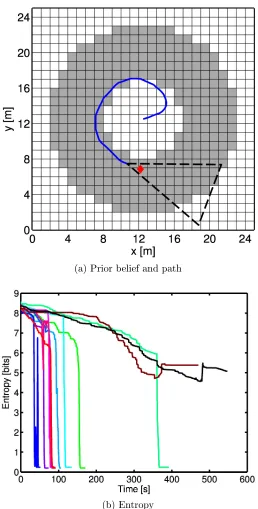
Figure 3: Illustration of our multi-robot multi-target localization algorithm. The robots (green squares) estimate the locations of targets (orange diamonds) and hazards (red dots) with high resolution by adaptively rening a cellular decomposition of the environment, despite having noisy sensors. The robots move to improve their estimate of the target locations while avoiding the estimated hazard locations by following the gradient of mutual information. The robots' nite sensor footprints (green circles) allow for decentralized estimation and control computations.

using the detections and failures of the robots in the team. The resolution of these cells is dynamically updated to provide ner localization of targets with limited computational resources. Using these estimates, the decentralized control algorithm moves the team of robots in the direction of greatest immediate information gain, a strategy sometimes called information surng [41]. More precisely, the controller moves the robots along the gradient of mutual information of target locations and measurements with respect to the positions of the robots. This implicitly tends to drive the robots to avoid hazardous areas as a failed robot provides no information, naturally merging the objectives of localizing targets and avoiding hazards.

The research in this chapter was originally published in [26, 27, 90].

3.1 Problem Formulation

Consider a situation wherenrobots move in a bounded, planar environmentE⊂_R2_{. Robot}

i is at position qi_t∈ E at time t, and the positions of all the robots can be written as the

stacked vector qt = [(q1t)T. . .(qnt)T]T. Each robot is equipped with a binary sensor which

(50)

Robots can also detect the failure status of other robots,fi∈ {0,1}, wherefi = 1 indicates that robotihas failed. Let the vector of sensor measurements be given byz= [z1, . . . , zn]T, wherez∈ {0,1}n₌_Z_{, and the vector of all failure statuses by}_f _{= [}_f1_{, . . . , f}n_]T _{∈ {}₀_,₁_}n_.

3.1.1 Map Representation

Finite set statistics (FISST) circumvents the issue of data association in target tracking by not implicitly (or explicitly) labeling individual targets. Rather than random vectors, FISST is based on random nite sets (RFSs), which are sets containing a random number of random elements describing the locations of each target. In this scenario, with the environment being represented by a collection of discrete cells, an RFS will be a set of labels of occupied cells. Due to the discretization of the environment in our case, the set integral will reduce to a nite sum. Also, the restriction that elements in an RFS be unique means that only one target may be within each cell, requiring the minimum cell size to be smaller than the minimum separation between objects. By employing an adaptive discretization of the environment, individual targets may be localized with high precision while empty areas are represented by a small number of large cells. Let the discretization representing target locations be denoted

{Es j}

mT

j=1 ⊂ E, where mT is the number of cells, and a set of target locations be X ∈ X,

whereXis the RFS for a given discretization. Similarly, another discretization{E_jh}mH j=1 ⊂E is used to represent the locations of hazards within the environment and a set of cell labels drawn from this discretization is denoted H∈H.

3.1.2 Sensor Models

As previously mentioned, the robots have a chance of failure due to hazards in the environ-ment. Let the probability of robot i, with pose qi, failing due to a hazard in cell E_jh be modeled by p(fi = 1 |j ∈H,qi) ≈α(qi, E_jh) while p(fi = 1 |j /∈H,qi) = 0. We assume that robot failures are conditionally independent given the locations of the hazards so

p(fi = 0|H,qi) = (1−pf) Y

j∈H

(51)

since the only way to not have a failure is to not fail due to any of the individual hazards or due to some other failure with probabilitypf(1). The probability of failure is then the additive complement of (3.1).

When a robot has failed, it provides no further information about the location of targets, leading to the conditional probability p(zi = 1 | fi = 1, X,qi) = 0. If a sensor is still functional, the detection equations are analogous to that of the hazards, beginning with

p(zi _{= 1} _| _fi _{= 0}_{, j} _∈ _X,_qi₎ _≈ _µ₍_qi_{, E}s

j) and p(zi = 1 | fi = 0, j /∈ X,qi) = 0. The

detections of each target are also conditionally independent given the target locations so

p(zi = 0|fi= 0, X, H,qi) = (1−pfp) Y

j∈X

p(zi= 0|fi = 0, j,qi), (3.2)

wherepfp is the probability of a false positive reading.

The failure model, p(fi = 1|j∈H,qi), and sensor model,p(zi = 1|fi= 0, j∈X,qi), of the robots have several key properties. First, real sensors have a nite eld of view, so these models should have compact support. Let Fi be the set of labels of cells within the footprint of robotiand consider the subset of RFSs containing targets inFi,Vi ={X ∈X|

x∈Fi _∀_x_∈_X_}_{. This is found using the projection} _ri

T :X→Vi given byrTi(X) =X∩Fi.

Note that this map is surjective but not injective as long as Fi is a proper subset of E, so no inverse mapping exists. The right inverse still exists, where ri_T((ri_T)−1(V)) =V but

(ri_T)−1(r_Ti (X))6=X. The right inverse of the projection is(ri_T)−1(V) ={X|r_Ti(X) =V},

which returns multiple values in general. Let Wi be the analogous neighborhood in the hazard grid with projectionri_H.

Second, the features may be located anywhere within the cell. Given this, the probability of failure due to a hazard in cellE_jh is given by

α(qi, E_jh) =

Z

Eh j

gh(qi,x)p(x)dx≈

1 m

m X

k=1

gh(qi,ehj,k), (3.3)

wheregh(qi,x)is a function describing the probability of failure due to a hazard at location