University of Pennsylvania
ScholarlyCommons
Publicly Accessible Penn Dissertations
1-1-2016
Planning With Adaptive Dimensionality
Kalin Vasilev Gochev
University of Pennsylvania, [email protected]
Follow this and additional works at:
http://repository.upenn.edu/edissertations
Part of the
Artificial Intelligence and Robotics Commons
, and the
Robotics Commons
This paper is posted at ScholarlyCommons.http://repository.upenn.edu/edissertations/1739 For more information, please [email protected].
Recommended Citation
Gochev, Kalin Vasilev, "Planning With Adaptive Dimensionality" (2016).Publicly Accessible Penn Dissertations. 1739.
Planning With Adaptive Dimensionality
Abstract
Modern systems, such as robots or virtual agents, need to be able to plan their actions in increasingly more complex and larger state-spaces, incorporating many degrees of freedom. However, these high-dimensional planning problems often have low-dimensional representations that describe the problem well throughout most of the state-space. For example, planning for manipulation can be represented by planning a trajectory for the end-effector combined with an inverse kinematics solver through obstacle-free areas of the
environment, while planning in the full joint space of the arm is only necessary in cluttered areas. Based on this observation, we have developed the framework for Planning with Adaptive Dimensionality, which makes effective use of state abstraction and dimensionality reduction in order to reduce the size and complexity of the state-space. It iteratively constructs and searches a hybrid state-space consisting of both abstract and non-abstract states. Initially the state-space consists only of non-abstract states, and regions of non-non-abstract states are selectively introduced into the state-space in order to maintain the feasibility of the resulting path and the strong theoretical guarantees of the algorithm---completeness and bounds on solution cost sub-optimality. The framework is able to make use of hierarchies of abstractions, as different abstractions can be more effective than others in different parts of the state-space. We have extended the framework to be able to utilize anytime and incremental graph search algorithms. Moreover, we have developed a novel general incremental graph search algorithm---tree-restoring weighted A*, which is able to minimize redundant computation between iterations while efficiently handling changes in the search graph. We have applied our framework to several different domains---navigation for unmanned aerial and ground vehicles, multi-robot collaborative navigation, manipulation and mobile manipulation, and navigation for humanoid robots.
Degree Type Dissertation
Degree Name
Doctor of Philosophy (PhD)
Graduate Group
Computer and Information Science
First Advisor Maxim Likhachev
Second Advisor Alla Safonova
Keywords
Subject Categories
PLANNING WITH ADAPTIVE DIMENSIONALITY
Kalin Vasilev Gochev
A DISSERTATION
in
Computer and Information Science
Presented to the Faculties of the University of Pennsylvania
in Partial Fulfillment of the Requirements for the
Degree of Doctor of Philosophy
2016
Supervisor of Dissertation
Maxim Likhachev
Adjunct Assistant Professor
Computer and Information Science
Co-Supervisor of Dissertation
Alla Safonova Assistant Professor
Computer and Information Science
Graduate Group Chairperson
Lyle Ungar Professor
Computer and Information Science
Dissertation Committee
Christopher Atkeson, Professor of Computer Science
Norman Badler, Professor of Computer and Information Science
Kostas Daniilidis, Professor of Computer and Information Science
PLANNING WITH ADAPTIVE DIMENSIONALITY
c
COPYRIGHT
2016
Kalin Vasilev Gochev
This work is licensed under the
Creative Commons Attribution
NonCommercial-ShareAlike 3.0
License
To view a copy of this license, visit
ABSTRACT
PLANNING WITH ADAPTIVE DIMENSIONALITY
Kalin Vasilev Gochev
Maxim Likhachev
Alla Safonova
Modern systems, such as robots or virtual agents, need to be able to plan their actions in
increasingly more complex and larger state-spaces, incorporating many degrees of freedom.
However, these high-dimensional planning problems often have low-dimensional
represen-tations that describe the problem well throughout most of the state-space. For example,
planning for manipulation can be represented by planning a trajectory for the end-effector
combined with an inverse kinematics solver through obstacle-free areas of the environment,
while planning in the full joint space of the arm is only necessary in cluttered areas. Based
on this observation, we have developed the framework for Planning with Adaptive
Dimen-sionality, which makes effective use of state abstraction and dimensionality reduction in
order to reduce the size and complexity of the state-space. It iteratively constructs and
searches a hybrid state-space consisting of both abstract and non-abstract states. Initially
the state-space consists only of abstract states, and regions of non-abstract states are
se-lectively introduced into the state-space in order to maintain the feasibility of the resulting
path and the strong theoretical guarantees of the algorithm—completeness and bounds on
solution cost sub-optimality. The framework is able to make use of hierarchies of
abstrac-tions, as different abstractions can be more effective than others in different parts of the
state-space. We have extended the framework to be able to utilize anytime and incremental
graph search algorithms. Moreover, we have developed a novel general incremental graph
search algorithm—tree-restoring weighted A*, which is able to minimize redundant
applied our framework to several different domains—navigation for unmanned aerial and
ground vehicles, multi-robot collaborative navigation, manipulation and mobile
TABLE OF CONTENTS
ABSTRACT . . . iii
LIST OF TABLES . . . viii
LIST OF ILLUSTRATIONS . . . x
CHAPTER 1 : Introduction . . . 1
CHAPTER 2 : Motivating Observation . . . 5
CHAPTER 3 : Related Work . . . 7
3.1 State Abstraction Techniques . . . 7
3.2 Two-Layer Planners . . . 9
3.3 Sampling-Based Planners . . . 10
3.4 Optimization Methods . . . 13
3.5 Incremental Search Algorithms . . . 13
CHAPTER 4 : Planning with Adaptive Dimensionality . . . 16
4.1 Definitions and Notations . . . 16
4.2 Overview . . . 17
4.3 Hybrid State-Space Construction . . . 20
4.4 Algorithm . . . 23
4.5 Identifying Areas that Require High-Dimensional Planning . . . 26
4.6 Theoretical Properties . . . 27
4.7 Algorithm Parameters . . . 29
CHAPTER 5 : Hierarchical Planning with Adaptive Dimensionality . . . 31
5.2 Related Work . . . 31
5.3 Combining Multiple Abstractions . . . 33
5.4 Theoretical Properties . . . 37
5.5 Identifying Useful Abstractions . . . 39
CHAPTER 6 : Incremental Graph Search forPAD . . . 46
6.1 Motivation . . . 46
6.2 Definitions and Notations . . . 48
6.3 Tree-Restoring Weighted A* Search . . . 48
6.4 Anytime Tree-Restoring Weighted A* Search . . . 55
6.5 Efficiently Detecting Changes in the Graph . . . 57
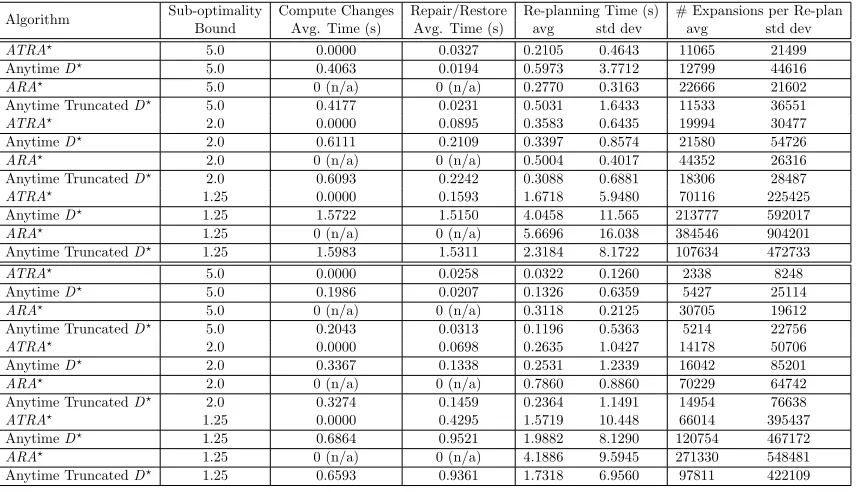
6.6 Experimental Evaluation . . . 58
6.7 Analysis of Results . . . 60
CHAPTER 7 : Application: PAD for Navigation . . . 65
7.1 Non-Incremental 3D Path Planning for a Non-Holonomic Vehicle . . . 65
7.2 Incremental 3D Path Planning for a Non-Holonomic Vehicle . . . 69
7.3 Interleaving Planning and Execution . . . 74
CHAPTER 8 : Application: PAD for Multi-Robot Collaborative Navigation . . . . 85
8.1 Related Work . . . 86
8.2 State Lattice with Controller-based Motion Primitives . . . 88
8.3 Implementation Details . . . 91
8.4 Experimental Setup . . . 97
8.5 Analysis of Results . . . 99
CHAPTER 9 : Application: PAD for Manipulation . . . 101
9.1 Using 3D Low-Dimensional Representation . . . 101
CHAPTER 10 : Application: PAD for Mobile Manipulation . . . 120
10.1 Using a Single Abstraction . . . 120
10.2 Using Multiple Abstractions . . . 125
CHAPTER 11 : Application: PAD for Humanoid Robot Mobility . . . 132
11.1 Domain Background and Related Work . . . 132
11.2 Algorithm Extension . . . 135
11.3 Implementation Details . . . 140
11.4 Experimental Evaluation . . . 150
11.5 Analysis of Results . . . 151
CHAPTER 12 : Conclusion . . . 154
APPENDIX . . . 156
LIST OF TABLES
TABLE 1 : Anytime TRA? simulation results . . . 60
TABLE 2 : Fixed sub-optimality TRA? simulation results . . . 61
TABLE 3 : Non-holonomic vehicle navigation planning . . . 68
TABLE 4 : Non-holonomic vehicle navigation planning on PR2 robot . . . 71
TABLE 5 : Incremental vs. non-incremental PAD for navigation . . . 72
TABLE 6 : Interleaving vs. non-interleaving PAD for navigation . . . 81
TABLE 7 : Results for multi-robot collaborative navigation planning . . . 99
TABLE 8 : Results for multi-robot collaborative navigation planning . . . 100
TABLE 9 : 7D/3D manipulation planning results . . . 105
TABLE 10 : Consistency comparison of search-based vs. sampling-based planners 106 TABLE 11 : 7D/4D manipulation planning results . . . 117
TABLE 12 : Path quality comparison results . . . 118
TABLE 13 : Performance of 7D/4D manipulation planning for independent wrist joints . . . 118
TABLE 14 : 11D/3D mobile manipulation results . . . 124
TABLE 15 : Manipulating a stick trough a window: 11D/7D adaptive planner vs. RRT planner results . . . 124
LIST OF ILLUSTRATIONS
FIGURE 1 : WeightedA∗ search example . . . 3
FIGURE 2 : Motivation example: navigation planning . . . 6
FIGURE 3 : Motivation example: motion planning . . . 6
FIGURE 4 : Example of an asymmetric cost function . . . 11
FIGURE 5 : Hybrid graph transitions . . . 18
FIGURE 6 : Planning with Adaptive Dimensionality in 3D/2D . . . 23
FIGURE 7 : Planning with Adaptive Dimensionality in 7D/3D . . . 24
FIGURE 8 : Transitions between abstract sub-spaces . . . 35
FIGURE 9 : Estimating cost gradient for graphs . . . 44
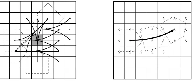
FIGURE 10 : Tree-restoringA? example . . . 49
FIGURE 11 : Computing affected graph edges from changed map cells . . . 57
FIGURE 12 : TRA? example environment . . . 58
FIGURE 13 : Example maps for non-holonomic vehicle navigation . . . 67
FIGURE 14 : Incremental Planning with Adaptive Dimensionality example . . . 70
FIGURE 15 : 3D/2D Planning with Adaptive Dimensionality for PR2 robot . . 71
FIGURE 16 : Number of iterations vs. speed-up factor . . . 72
FIGURE 17 : PR2 in a cluttered indoor environment. . . 80
FIGURE 18 : Example graph using state-lattice controllers . . . 90
FIGURE 19 : Multi-robot adaptive navigation planning example . . . 94
FIGURE 20 : Robots used for multi-robot collaborative navigation . . . 96
FIGURE 21 : Maps used in multi-robot collaborative navigation . . . 99
FIGURE 23 : Manipulation planning example environments . . . 103
FIGURE 24 : Trajectory being executed by actual PR2 robot . . . 105
FIGURE 25 : 7D/4D manipulation planning example . . . 109
FIGURE 26 : Heuristic local minimum example . . . 113
FIGURE 27 : PR2 retrieving an object from a fridge . . . 116
FIGURE 28 : Degrees of freedom for mobile manipulation on PR2 robot . . . . 121
FIGURE 29 : PR2 manipulating a stick trough a window . . . 122
FIGURE 30 : PR2 reaching from a high shelf to a low shelf of a bookcase . . . . 122
FIGURE 31 : Example kitchen environment . . . 128
FIGURE 32 : Example indoor environment from real sensor data . . . 128
FIGURE 33 : Planning phase of Planning with Adaptive Dimensionality with multiple abstractions . . . 129
FIGURE 34 : Tracking phase of Planning with Adaptive Dimensionality with multiple abstractions . . . 130
FIGURE 35 : Initial distribution of sub-spaces in environment . . . 130
FIGURE 36 : Humanoid Robots . . . 133
FIGURE 37 : Humanoid Mobility Example . . . 134
FIGURE 38 : Yamabiko Humanoid Robot . . . 140
FIGURE 39 : Humanoid Robot Abstraction Hierarchy . . . 141
FIGURE 40 : Bipedal Abstraction for Flat Terrain . . . 143
FIGURE 41 : Bipedal Abstraction for Stairs . . . 144
FIGURE 42 : Maintaining Static Stability . . . 147
CHAPTER 1 : Introduction
Planning is an important component of any intelligent system. It allows the system to adapt
to changing environment conditions and sensory inputs. In recent years robotics research
has moved from the controlled predictable industrial environments towards the cluttered,
uncontrolled and unpredictable domestic environments, where robots need to be able to
safely perform a variety of tasks necessitating careful, but efficient, planning. Search-based
planning algorithms are often used in many areas of robotics and artificial intelligence. They
represent the planning problem as a graph search in a graph consisting of a set of nodes,
denoting valid system configurations, and a set of edges, denoting valid transitions from
one system configuration to another. The planning problem then becomes finding a path (a
sequence of edges) in the graph from a given start node to a given goal node. Henceforth,
we will refer to nodes in a graph as system states, or simply states, and to the set of nodes
in a graph as the state-space.
The most common application of search-based planning is navigation planning or
path-finding (Likhachev and Ferguson, 2008; Dolgov et al., 2010). It is also commonly used
to solve discrete combinatorial problems, such as various puzzles and games (Holte et al.,
1996b). There are several important reasons for the popularity of search-based planners.
Firstly, they typically provide strong theoretical guarantees on completeness with respect
to the graph representing the search problem, and bounds on solution cost sub-optimality.
Usually, in search-based planners one can easily trade-off solution optimality for faster
plan-ning time, for example, by varying the heuristic weighting factor in Weighted A* search,
and still have strong guarantees that the cost of the solution is within a desired bound
of the optimal solution cost. Second, a number of anytime search algorithms have been
developed, that find the best solution they can within a given time limit and continue to
improve the solution quality as the planning time allows (ARA* (Likhachev et al., 2003),
Anytime A* (Zhou and Hansen, 2002), Beam-Stack Search (Zhou and Hansen, 2005b)).
solu-tions faster (Focussed D* (Stentz, 1995a), Incremental A* (Koenig and Likhachev, 2002b),
D* Lite (Koenig and Likhachev, 2002a)). Such algorithms are well-suited for planning in
dynamic environments, where fast re-planning is necessary. Finally, formulating the search
problem as a cost-minimization problem allows one to define and incorporate complex cost
functions and constraints into the planning process. These properties of search-based
plan-ning algorithms address common considerations when desigplan-ning intelligent systems, such as
efficiency, response time, and consistency.
Modern intelligent systems, such as robots or virtual agents, need to be able to plan their
actions in increasingly more complex state-spaces with many degrees of freedom. These
degrees of freedom are often introduced to capture the full capabilities of the system, or to
account for its various kinodynamic constraints. In the context of search-based planning,
the increasing number of degrees of freedom of the system introduces an exponential increase
in the size of the search space, also known as the “curse of dimensionality”. Thus, the high
dimensionality of the states-space often leads to a dramatic increase in the time and memory
required by the search algorithm to find a solution. Dijkstra’s graph search algorithm
(Dijkstra, 1959) is probably the most well-known graph search algorithm with running time
of about O(|E|log(|V|)), depending on the specific implementation, where E is the set of
edges andV is the set of nodes in the graph. However, this running time becomes impractical
for systems with large number of degrees of freedom, as|V|and|E|scale exponentially with
the number of degrees of freedom.
Search-based algorithms try to alleviate the problem by focusing the search efforts in
promising directions by using heuristic functions (or simply heuristics) (Hart et al., 1968)—
functions that estimate the cost of reaching the goal from every state in the search space.
A heuristic is said to be admissible if it never overestimates the cost of reaching the goal.
Usually, admissible heuristics are required in order for the search-based planning algorithms
to provide guarantees about the cost of the solution. However, some algorithms impose an
Figure 1: WeightedA∗ search (= 5) on an 8-connected 2D grid using Euclidean distance cost between nodes from start (bottom left) to goal (top right). The heuristic used is Euclidean distance to the goal. The gray shape represents an obstacle. Blue circles represent nodes on the OPEN list, solid colored nodes represent expanded nodes, with color varying from red to green based on increasing g value. Solid blue nodes are invalid nodes that are in collision with the obstacle. The green path represents the solution to the problem found by the weighted A∗ search. The shape of the obstacle introduces a local minimum of the heuristic function. All nodes in the local minimum are expanded by the search. Image taken from (Wikipedia, 2015).
heuristichis said to be consistent (or monotone) if and only if it is admissible and obeys the
triangle inequality for any stateA in the state-spaceS and any state B ∈successors(A):
h(A)≤cost(A, B) +h(B) ∀A∈S,∀B ∈successors(A).
These limitations on the heuristic functions, combined with the increasing complexity of
the search problems being studied, make it very challenging for researchers to find good
heuristics that perform well over a wide range of problems. It is often challenging to find
heuristics that perform consistently over a wide variety of problem instances. Pronounced
local minima in the heuristic can lead to a significant performance decrease, as the search
needs to expand all states in the local minimum in order to overcome it and proceed towards
the goal (Fig. 1). In Fig. 1, the heuristic does not take into account obstacles in the search
space, and thus, certain obstacle shapes and configurations can produce very large local
We have developed a framework for search-based planning, Planning with Adaptive
Dimen-sionality (PAD), that tries to address the size of the state-space and the “curse of
dimension-ality” for high-dimensional planning problems based on the observation described in the next
chapter. We demonstrate that the framework provides the important theoretical properties
of search-based planning algorithms—completeness with respect to the graph
represent-ing the problem and strong guarantees on solution cost sub-optimality bounds. We have
also experimentally validated our framework in a number of planning domains—navigation,
CHAPTER 2 : Motivating Observation
While planning in a high-dimensional state-space is often necessary to capture the full
ca-pabilities of the system and its kinodynamic constraints, large portions of the computed
solutions exhibit low-dimensional structures. For example, a 3-DoF (x,y,heading) path for
a non-holonomic vehicle typically contains large portions that are straight-line segments
and do not therefore require three-dimensional planning. On the other hand, sections of
the path that include turning do require planning in all three degrees of freedom in order to
capture the minimum turning radius constraints of the system (Fig. 2). Similarly, planning
for manipulation can often be reduced to 3-DoF (x, y, z) planning for the manipulator’s
end-effector position and using an inverse kinematics solver to find a full-dimensional
ma-nipulator path that corresponds to the computed end-effector path (Fig. 3 (a)). At the
same time, there are situations when the planner does need to consider the full
configu-ration of the arm when trying to ensure the feasibility of the end-effector path—in highly
cluttered areas of the environment or certain obstacle configurations (Fig. 3 (b)), for
ex-ample. Such low-dimensional representations can be found for many robotic systems, as
they are inherently embedded into the 2D planar or 3D spatial geometric environments in
which they operate. Moreover, a number of informative heuristics exist for such geometric
environments, such as various distance metrics, which can even account for the obstacles in
the environment. Thus, search in these low-dimensional spaces can be performed quickly
and efficiently.
In this work, we present an algorithm framework that exploits this observation. It
itera-tively constructs a hybrid state-space that utilizes a low-dimensional state representation
(abstraction) throughout most of the search space (e.g. end-effector position), except for
the areas where low-dimensional planning fails and full-dimensional planning is necessary
(e.g. full manipulator configuration) to ensure that the solution is feasible and satisfies a
desired cost sub-optimality bound. At each iteration the algorithm identifies areas of the
Figure 2: Example trajectory for a non-holonomic vehicle with minimum turning radius constraints. Planning for the heading of the vehicle is needed in areas that require turning in order to ensure constraints are satisfied (light red circles). Planning for the heading of the vehicle is unnecessary for areas that can be traversed in a straight line. A: start location; B: goal location; gray boxes: obstacles.
(a) (b)
Figure 3: Motion planning for a manipulator: (a) Simple example: planning an end-effector trajectory and using an inverse kinematics solver to compute a corresponding manipulator trajectory. (b) Example: planning an end-effector trajectory combined with an inverse kinematics solver fails to produce a valid trajectory.
graph, until the necessary high-dimensional areas have been identified and the planner is
able to compute a feasible solution. Using such low-dimensional abstractions results in
sub-stantial reduction in the size of the state-space and considerable speedups in planning time
and lower memory requirements of the planner. On the theoretical side, we have shown that
the method is complete with respect to the state-space representing the search problem and
can provably guarantee to find a solution, if one exists, within a desired cost sub-optimality
bound. Additionally, we present a number of extensions of the framework that can further
CHAPTER 3 : Related Work
In order to improve planning times and memory requirements, researchers have used a
variety of techniques to avoid performing global planning in large high-dimensional
state-spaces.
3.1. State Abstraction Techniques
State abstraction is a general technique for simplifying search problems by reducing the size
and complexity of the search space. The general idea is to combine states in the original
state-space into abstract states based on pre-defined set of criteria, thus creating a much
smaller abstract state-space. A search is then performed on the abstract state-space and
the results of the search are used to guide a subsequent search of the original state-space. In
other words, abstraction provides a means of automatically creating admissible heuristics
for graph search algorithms and has been studied by researchers since the 70’s (Guida and
Somalvico, 1978; Gaschnig, 1979; Pearl, 1984; Prieditis, 1993). In order for the abstraction
to generate an admissible heuristic, the distance between every pair of states A and B in
the original state-space S must be no less than the distance between their corresponding
abstract statesA0 andB0 in the abstract state-spaceS0 (i.e. the abstraction underestimates
distances or costs between states).
cost(A, B)≥cost(A0, B0)∀A, B∈S
A0=image(A)∈S0, B0 =image(B)∈S0
Different hierarchical planners use different methods of abstraction to make better-informed
heuristics to guide the search, such as the clique abstraction in (Bulitko et al., 2007) and
the max-degree star abstraction in (Holte et al., 1996a,b). The most important difference
informative heuristic functions, our approach focuses on removing irrelevant dimensions
from the planning process itself. These dimensions are only considered in regions of the
state-space that require them in order to ensure the feasibility of the resulting solution
and its cost sub-optimality bound. Moreover, the abstractions considered by hierarchical
planners (Holte et al., 1996b,a; Botea et al., 2004; Bulitko et al., 2007) usually combine
states that are adjacent or within a certain distance in terms of number of edges within the
state-space. Usually, such abstractions require the full graph representing the state-space
to be constructed and stored in memory, which may be infeasible in many high-dimensional
systems. Then the abstract graph is constructed and used to compute a heuristic for the
problem instance in a pre-processing step that can be quite computationally expensive.
Thus, these approaches are not well-suited for dynamic environments. Both the clique
(Bulitko et al., 2007) and max-degree star (Holte et al., 1996a,b) abstractions require
sig-nificant pre-processing. In addition, computing the clique abstraction in a general graph
is an NP-complete problem. Bulitko et al. (Bulitko et al., 2007) are able to compute the
abstraction efficiently only in 8-connected 2D grids. In contrast, our method uses projection
functions to project states to and from the low-dimensional state-space. This allows us to
dynamically construct both the low-dimensional and high-dimensional regions of the graph,
and thus, we do not need to pre-allocate memory for the entire graph.
Our approach is also somewhat relevant to planners that use very accurate pre-computed
heuristic values (Knepper and Kelly, 2006). Similarly to the hierarchical planners using
state abstraction, the heuristics are often derived by solving a simplified lower-dimensional
problem. As a result, these methods can be viewed as full-dimensional planning that uses
the results of lower dimensional planning. Unlike our approach however, these methods do
not explicitly decrease the dimensionality and, as a result, can run into severe computational
problems when the heuristic is inaccurate. As mentioned above, our approach does not focus
on computing accurate heuristics, but rather decreases the dimensionality of the problem in
order to explicitly reduce the size of the state-space. In addition, our framework for Planning
to the reduced size of the state-space, our approach is more robust to handling possible
heuristic local minima than approaches that perform full-dimensional planning. Thus, the
performance of our approach does not rely solely on the quality of the heuristic.
Kapadia et al. (Kapadia et al., 2013) use an approach very similar to ours. They use
the same concept of a “tunnel” around a low-dimensional path, which we introduce in the
following chapter, to focus and constrain a subsequent search of a high-dimensional space.
They also incorporate multiple low-dimensional representations in their planning framework
to form an abstraction hierarchy, which we discuss in Chapter 5, and use an incremental
graph search algorithm to speed-up subsequent search queries, which we discuss in Chapter
6. Their approach, however, is significantly different than ours in that they do not use
hybrid graphs containing both low- and high-dimensional states, which we use to ensure
the completeness of our algorithm and that the desired cost sub-optimality bound is met.
In contrast, their approach relies on increasing the width of the “tunnel” until a valid
high-dimensional path is found through it. Moreover, their approach does not provide bounds
on the solution cost sub-optimality.
3.2. Two-Layer Planners
Many path planners implement a two layer planning scheme, where a low-dimensional global
planner provides input to a high-dimensional local planner. Since these local planners
operate on a small subset of the entire environment, usually in the immediate vicinity of
the robot, they can afford to incorporate more dimensions, while still meeting planning time
constraints. The local planners have been implemented using reactive obstacle avoidance
planners (Thrun et al., 1998) and dynamic windows (Philippsen and Siegwart, 2003; Brock
and Khatib, 1999) to produce feasible paths from an underlying low-dimensional global
planner. However, these techniques can result in highly sub-optimal paths and even paths
that are infeasible for execution by the system due to mismatches in the assumptions made
by the global and the local planners. In contrast, our approach does not split the planning
problem within a single planning process. By combining the abstract and non-abstract state
representations in a single hybrid graph, our framework is able to identify areas exhibiting
inconsistencies between the low-dimensional and high-dimensional state representations and
remedy these inconsistencies by requiring high-dimensional planning to be performed in
those areas. Moreover, our approach is complete with respect to the full-dimensional
state-space and guarantees to compute a path that is feasible in the full-dimensional state-state-space
if one exists.
3.3. Sampling-Based Planners
Sampling-based motion planners, such as probabilistic roadmaps (PRM) (Kavraki et al.,
1996; Bohlin and Kavraki, 2000), and rapidly-exploring random trees (RRT) (LaValle and
Kuffner, 2001a) and its variants (Kuffner and LaValle, 2000; Berenson et al., 2009, 2011;
Karaman et al., 2011) have become extremely popular in recent years for solving
high-dimensional planning problems. They have been shown to solve impressive high-high-dimensional
motion planning problems, while being simple, fast, and easy to implement. These methods
have also been extended to support motion constraints through rejection sampling (Sucan
and Kavraki, 2009).
Our search-based approach to planning differs from the sampling-based methods in
sev-eral important aspects. First, sampling-based motion planners are mainly concerned with
finding any feasible path, rather than minimizing the cost of a solution. The notable
ex-ception is the RRT* algorithm (Karaman et al., 2011), which asymptotically converges to
an optimal solution and is one of the algorithms that we compare our approach against
ex-perimentally. In general, sampling-based approaches sacrifice cost minimization in order to
gain very fast planning speeds. As such, they may often produce solutions of unpredictable
length involving highly sub-optimal or jerky motions that may be hard for the system to
execute. To compensate for the lack of solution cost minimization, sampling-based methods
rely on various smoothing techniques to improve the quality of the computed trajectory.
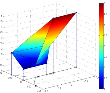
meth-Figure 4: Example of an asymmetric cost function: energy consumption effect of changing altitude for a UAV. Transitioning from state A to state B (red arrow) is more costly than transitioning from state B to state A (blue arrow). Thus, in terms of cost, moving from B to A is closer than moving from A to B, which makes the cost function not a proper distance metric. Such cost functions present a challenge for sampling-based algorithms.
ods which aim to provide solution cost minimization, such as RRT*, usually have to use
a distance metric for their cost function and do not support arbitrary cost functions, due
to the requirement for solving k-nearest neighbors queries in the cost space. However, in
robotics cost functions are often non-symmetric, which violates the distance metric
require-ments. In many systems the cost of transitioning from stateAto state B is not necessarily
equal to the cost of transitioning from B toAin the state-spaceS.
∃A, B ∈S s.t. cost(A, B)6=cost(B, A)
For example, the energy consumption for a unmanned aerial vehicle (UAV) is higher for
increasing altitude than it is for decreasing altitude (Fig. 4). Thus, if the cost function is
based on energy consumption, the costs of actions that involve changes in altitude are highly
asymmetric. Moreover, it is generally much easier and safer for a robot to move forward
than backward, as sensors are usually located at the front of the robot. Thus, moving
backward is often considered undesirable and such actions are associated with much higher
easily handled by search-based planners by using a directed graph to represent the problem.
Another difference between and sampling-based planning methods is that
search-based planners produce more consistent solutions between planning episodes with similar
start and goal configurations. Due to their randomized nature, sampling-based methods
may often produce solutions of unpredictable length that can be inconsistent from one
planning episode to another. It is often preferable for planners to produce similar solutions
for planning queries with similar start/goal configurations. Consistency of planners is an
important consideration when the system needs to operate in environments with proximity
to humans. Humans need to be able to predict and anticipate the behavior of the system
in order to feel safe and comfortable around it. In our experimental evaluation we compute
a consistency measure of the trajectories produced by our approach and sampling-based
alternatives and compare the results.
Finally, the performance of sampling-based methods can suffer significantly in very cluttered
environments with narrow solution spaces. Researchers have tried to address this problem
by developing non-uniform sampling techniques that try to identify narrow passages and
bias sampling in those areas (Lee et al., 2012). However, one must be very careful how
one biases the sampling, as biased sampling can often break the algorithm’s probabilistic
completeness, and in the case of RRT*, even its guarantee to converge to optimality.
There are certain similarities between search- and sampling-based methods. For example,
methods based on PRM (Kavraki et al., 1996) only differ from search-based methods in the
way the underlying graph is constructed. PRM-based methods use sampling to generate
nodes in the graph, rather than regular discretization of the continuous space. However,
both PRM methods and search-based methods rely on efficient graph search algorithms in
3.4. Optimization Methods
Several motion planning algorithms have been developed that also try to minimize the
cost of solutions through optimization techniques (Ratliff et al., 2009; Kalakrishnan et al.,
2011). The Covariant Hamiltonian Optimization and Motion Planning (CHOMP) algorithm
(Ratliff et al., 2009) works by creating a naive initial trajectory from start to goal, and then
uses a method similar to gradient descent to try to minimize the cost function. The use
of gradient descent, however, makes the approach vulnerable to local minima in the cost
function. The final solution of the algorithm usually lies in the same homotopic class as
the initial estimate. Thus, the approach needs an initial solution estimate that is fairly
close to the optimal in order to converge to global optimality. The Stochastic Trajectory
Optimization for Motion Planning (STOMP) algorithm (Kalakrishnan et al., 2011), on the
other hand, relies on generating noisy trajectories to explore the space around a naive initial
trajectory. It then iteratively combines these trajectories to produce an updated trajectory
with lower cost. A cost function based on a combination of obstacle avoidance and path
smoothness is optimized in each iteration. The stochastic nature of the approach makes it
less vulnerable to local minima in the cost function, but does not guarantee convergence to
global optimality.
3.5. Incremental Search Algorithms
Researchers have developed various methods for performing incremental heuristic searches,
based on the observation that information computed during previous search queries can be
used to perform the current search faster. Due to its iterative nature, our framework for
Planning with Adaptive Dimensionality can benefit greatly from incremental graph search
algorithms in order to minimize redundant computation between iterations. Generally,
incremental heuristic search algorithms fall into three categories.
Anytime Truncated D? (Aine and Likhachev, 2013), aim to identify and repair inconsis-tencies in a previously-generated search tree. These approaches are very general and don’t
make limiting assumptions about the structure or behavior of the underlying graph. They
also demonstrate excellent performance by repairing search tree inconsistencies that are
relevant to the current search task. The main drawback of these algorithms is the
book-keeping overhead required, which sometimes may significantly offset the benefits of avoiding
redundant computation.
The second class of algorithms, such as Fringe-SavingA? (Sun et al., 2009) and Differential A? (Trovato and Dorst, 2002), also try to re-use a previously-generated search tree, but rather than attempting to repair it, these approaches aim to identify the largest portion of
the search tree that is unaffected by the changes and still valid, and resume searching from
there. These approaches tend to be less general and to make limiting assumptions about
the graph on which they operate. The Fringe-Saving A?, for example, only works on 2D grids with unit cost transitions between neighboring cells. It uses geometric techniques to
reconstruct the search frontier based on the 2D grid structure of the graph. The assumptions
made by these algorithms allow them to perform very well in scenarios that meet these
limiting assumptions.
The third class of incremental heuristic search algorithms, such as Generalized AdaptiveA? (Sun et al., 2008), aim to compute more accurate heuristic values by using information from
previous searches. As the heuristic becomes more informative, search tasks are performed
faster. The main challenge for such algorithms is maintaining the admissibility or
consis-tency of the heuristic when edge costs are allowed to decrease. Path- and Tree-Adaptive
A? (Hern´andez et al., 2011) algorithms, for example, rely on the fact that optimal search
is performed on the graph and edge costs are only allowed to increase. However, often in
robotics incremental search algorithms need to be able to support both increasing and
de-creasing edge costs to capture obstacles appearing and disappearing from the environment.
the environment. Moreover, performing optimal search is often impractical for systems with
a large number of degrees of freedom, making approaches that allow for trade-off between
solution quality and planning time more appealing for such systems.
We have developed a novel general anytime incremental graph search algorithm that works
well with our framework for Planning with Adaptive Dimensionality. We call the algorithm
Tree-Restoring Weighted A? and it falls into the second class of incremental search
algo-rithms described above, which identify and reuse valid portions of the search tree generated
by the previous search iteration. However, our approach differs from similar techniques in
that we do not make any limiting assumptions about the structure of the graph or the
be-havior of the cost function. Our algorithm is able to support both increasing and decreasing
edge costs on arbitrary graphs. The algorithm is an extension to the Anytime Repairing
A? (ARA?) algorithm (Likhachev et al., 2003) and has the same strong theoretical proper-ties, such as completeness and provable bounds on solution cost sub-optimality. Similarly
toARA?, our algorithm allows for trading-off between solution quality and planning time. Moreover, the algorithm has much lower book-keeping overhead when compared to
CHAPTER 4 : Planning with Adaptive Dimensionality
In this chapter we provide a detailed description of our algorithm for Planning with Adaptive
Dimensionality (PAD). We begin by introducing the important assumptions, definitions,
and notations used.
4.1. Definitions and Notations
We assume that the planning problem is represented by a discretized finite state-space S
of dimensionality d, consisting of states represented by state-vectorsX = (x1, ..., xd), and
a set of transitions T ={(Xi, Xj)|Xi, Xj ∈S}. Each transition (Xi, Xj) corresponds to a
feasible transition between the corresponding state vector values and is associated with a
cost c(Xi, Xj) which is bounded from below by some positive δ, that is,c(Xi, Xj)> δ >0.
Thus, we have an edge-weighted directed graphGwith a vertex setSand edge setT. We will
use the notationπG(Xi, Xj) to denote a path in graphGfrom stateXi to stateXj. The cost
of any pathπG(Xi, Xj) is the cumulative costs of the transitions along it and will be denoted
byc(πG(Xi, Xj)). We will useπ∗G(Xi, Xj) to denote a least-cost path andπG(Xi, Xj), ≥1
to denote a path of bounded cost sub-optimality c(πG(Xi, Xj)) ≤ ·c(π∗G(Xi, Xj)). The
goal of the planner is to find a least-cost path inGfrom the start stateXS to the goal state
XG. Alternatively, given a desired sub-optimality bound ≥1, the goal of the planner is
to find a path πG(XS, XG).
Definition 4.1 A heuristic function his said to beadmissiblefor a graph search problem
on an edge-weighted graph G and a goal stateg∈G if
h(s)≤c(π∗G(s, g))∀s∈G
i.e. the heuristic never overestimates the optimal cost of reaching the goal. Such heuristic
functions are sometimes called optimistic.
search problem on an edge-weighted graph G and a goal stateg∈Gif
h(s)≤c(s, t) +h(t)∀s∈G,∀t∈successors(s)
h(g) = 0
4.2. Overview
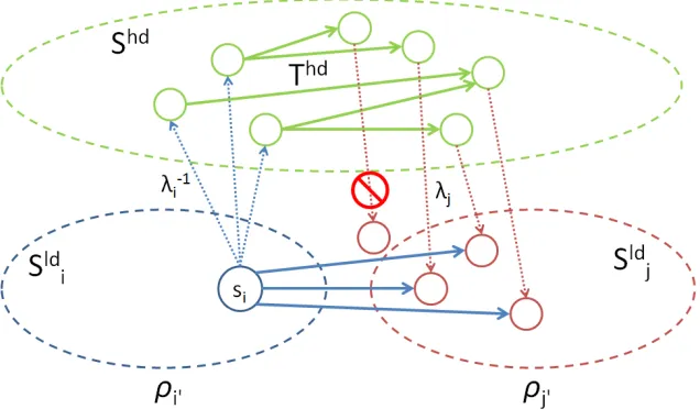
Let us consider two state-spaces—a high-dimensional SHD with dimensionality h, and a low-dimensional SLD with dimensionality l, which is a projection of SHD onto a lower dimensional manifold (h > l,|SHD|>|SLD|). We define a many-to-one mapping
λ:SHD →SLD
from the high-dimensional state-space SHD to the low-dimensional state-space SLD. For example, in the case of navigation planning for a non-holonomic vehicle in 3 dimensions (x,
y, heading) described in Chapter 7 we used a 2-dimensional state representation (x,y) and
the simple mapping λ((x, y, θ)) = (x, y), just dropping the heading information θfrom the
state-vector for low-dimensional states.
We also define the mapping λ−1 : SLD → (SHD)∗ from the low-dimensional state-space SLD to subsets of the high-dimensional state-spaceSHD, defined by
λ−1(XLD) ={X ∈SHD|λ(X) =XLD}
Notice that λ−1 is a one-to-many mapping and produces a set of high-dimensional states
corresponding to a given low-dimensional stateXLD—the set of pre-images of XLD.
Each of the two state-spaces may have its own transition set. For example, in the 3D/2D
navigation planning scenario described in Chapter 7 we used 8-connected 2D grid transitions
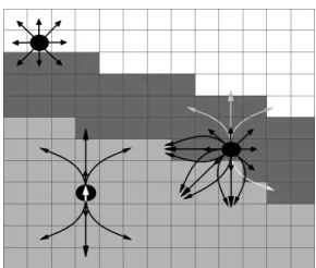
Figure 5: Example state transitions for a 3D/2D state-space–white cells are 2D states (x, y), dark gray cells are 2D states with feasible 3D transitions to 3D states (x, y,heading), and the light gray cells are 3D states. On the upper left is shown a 2D state with all of its feasible transitions (only 2D transitions). The state in the middle right is in the boundary area, so its feasible transitions include all 2D transitions that end in a 2D state and all 3D transitions (from all possible heading values) that end in a 3D state. In light gray are shown some of the disallowed 3D transitions, since they lead to 2D states. In the lower left is a 3D state with all of its 3D transitions (heading indicated by the white arrow).
kinodynamic constraints of the vehicle, called motion primitives (Likhachev and Ferguson,
2008), as transitions for the 3D state-space (Fig. 5).
Let GHD and GLD denote the corresponding graphs defined by SHD and SLD and their respective transition sets THD and TLD.
The idea of our algorithm is to iteratively construct and search a hybrid graph GAD con-sisting of both low- and high-dimensional states and transitions. InitiallyGAD is identical to GLD. The iterative nature of the algorithm stems from the fact that each iteration identifies new areas of GAD where high-dimensional regions need to be introduced until a valid solution is found. Upon addition of new high-dimensional regions intoGAD, another search iteration is performed on the new instance ofGAD taking into account the new
high-dimensional regions. The process is repeated until a search iteration is able to successfully
compute a solution that is feasible in the high-dimensional state-space and satisfies the
specified cost sub-optimality bound. We discuss the structure and the construction ofGAD below.
costs of the transitions inTHD andTLD be such that for every pair of states Xi andXj in
SHD,
c(π∗(Xi, Xj))≥c(π∗(λ(Xi), λ(Xj))) (4.1)
That is, we require that the cost of a least-cost path between any two states in the
high-dimensional state-space to be at least the cost of a least-cost path between their images
in the low-dimensional state-space. The intuition behind this requirement is that path
segments through the low-dimensional areas of the state-space provide optimistic estimates
of the true cost of their high-dimensional images. These optimistic estimates are used to
establish a lower bound on the overall optimal solution cost. The algorithm then uses this
lower bound to ensure that the final solution cost is within the desired sub-optimality factor
of the optimal solution cost.
Then let us formally define a state-abstraction in the context of Planning with Adaptive
Dimensionality as follows:
Definition 4.3 A state-abstraction of a state-space SHD is a tuple A = (λ, λ−1, GLD = (SLD, TLD), c), where:
• SLD is a projection of SHD to a lower-dimensional sub-space of SHD through a
pro-jection functionλ:SHD→SLD
• λ−1 :SLD →(SHD)∗ is defined as λ−1(XLD) ={X ∈SHD|λ(X) =XLD}
• GLD = (SLD, TLD) is an edge-weighted (directed) graph with vertex set SLD and
transition set TLD
• c:TLD →R+ is a cost function satisfying 4.1
When referring to the full-dimensional abstraction, we mean the identity abstraction of the
λ−1HD are both equal to the identity mapping over SHD (∀X ∈ SHD λHD(X) = X and
λ−1HD(X) ={X}).
4.3. Hybrid State-Space Construction
4.3.1. Structure of the Hybrid Graph
Recall that the goal of our algorithm was to use the faster low-dimensional planning, except
for areas of the environment where high-dimensional planning is necessary to ensure the
feasibility of the resulting path and the desired cost sub-optimality bound. We want our
hybrid state-space to capture this property—namely, we want GAD to consist largely of low-dimensional states, except for the areas where high-dimensional planning needs to be
performed, represented by areas of high-dimensional states inGAD. To ensure path feasibil-ity in the high-dimensional regions ofGAD, we have to use high-dimensional transitions. In the low-dimensional areas we can use simpler low-dimensional transitions. However, recall
that the transitions we have in THD andTLD connect two states of the same dimensional-ity, which do not allow us to transition from the low-dimensional to the high-dimensional
regions. Therefore, we have to construct a transition set TAD that allows for transitions between states of different dimensionality.
4.3.2. Construction of the Hybrid Graph
Our algorithm iteratively constructs GAD, beginning with the low-dimensional state-space SLDand introducing a set of high-dimensional regionsRin it. We first explain how the
high-dimensional regions are being introduced intoGADand connected with the low-dimensional regions. The algorithm that decides when and where to introduce these regions will be
explained later.
low-dimensional and high-low-dimensional states. Notice that if a high-low-dimensional stateXHD is in SAD, then its low-dimensional projectionλ(XHD) is not in SAD, and also ifXHD 6∈SAD, then λ(XHD) ∈ SAD. Thus, for every state XHD in the original high-dimensional state-space, eitherXHD∈SADorλ(XHD)∈SAD (but not both). Adding new high-dimensional regions or increasing the sizes of existing regions requires the reconstruction of SAD and TAD, and thus, will produce a new instance ofGAD = (SAD, TAD).
Next we define the transition set TAD for the hybrid graph GAD as follows.
Definition 4.4 Transitions in GAD: For any state Xi ∈SAD:
• If Xi is high-dimensional (Xi ∈ SHD), then for all high-dimensional transitions
(Xi, XjHD) ∈ THD, if XjHD ∈ SAD then (Xi, XjHD) ∈ TAD. If XjHD 6∈ SAD,
then (Xi, λ(XjHD))∈TAD. That is, for dimensional states we allow only
high-dimensional transitions to other high-high-dimensional states if they fall inside SAD, or their low-dimensional projections (Fig. 5 lower left).
• If Xi is low-dimensional (Xi ∈ SLD), then for all low-dimensional transitions
(Xi, XjLD)∈TLD, ifXjLD ∈SAD then(Xi, XjLD)∈TAD and for all high-dimensional
transitions (X, XjHD)∈THD, where X ∈λ−1(Xi), if XjHD ∈SAD then(Xi, XjHD)∈
TAD. That is, for low-dimensional states we allow low-dimensional transitions if they lead to another low-dimensional state inSAD(Fig. 5 upper left), and high-dimensional transitions from their high-dimensional projections if they lead to a high-dimensional
state inSAD (Fig. 5 right).
Notice, that the above definition of TAD allows for transitions between states of different
dimensionality. Figure 5 illustrates the set of transitions in the adaptive graph in the case
4.3.3. Mapping Hybrid Solutions to the High-Dimensional State-Space
Once we have computed a path through our hybrid graph GAD, which can contain
low-dimensional states and transitions, we need to be able to project it to the high-low-dimensional
state-space in order to ensure that it is feasible and satisfies the desired solution cost
sub-optimality bound. Therefore, we define a tunnel τ of radius w around a hybrid path πAD
as follows:
Definition 4.5 A tunnelτ of widthwaround a hybrid pathπADis a sub-graphτ = (Sτ, Tτ)
τ ⊆GHD such that
Sτ ⊆SHD
Tτ ⊆THD
∀XHD ∈SHD, XHD ∈Sτ iff ∃Xi ∈πAD s.t.
dist(λ(XHD), Xi)≤w if Xi ∈SLD or
dist(λ(XHD), λ(Xi))≤w if Xi ∈SHD
∀EHD= (Xi, Xj)∈THD, EHD ∈Tτ iff Xi ∈τ and Xj ∈τ
where dist is some pre-defined distance metric in SLD.
In other words,τ is a sub-graph ofGHD, and thus consists only of high-dimensional states and transitions. Moreover, τ contains all high-dimensional states XHD if they fall within distance w of some state Xi ∈ πAD. We include in τ all transitions (Xj, Xk) from THD
such that both Xj and Xk are in τ. It is important to note that the above definition of τ
for tunnel width w = 0 becomes equivalent to the sub-graph produced by projecting the
hybrid path πAD to the high-dimensional state-space SHD through the projection function
λ−1. This λ−1 projection method can be used when no distance metric is available in
the low-dimensional state-space. The above definition, however, allows for more flexibility
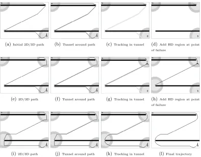
high-(a)Initial 2D/3D path (b) Tunnel around path (c) Tracking in tunnel (d) Add HD region at point of failure
(e)2D/3D path (f) Tunnel around path (g)Tracking in tunnel (h) Add HD region at point of failure
(i)2D/3D path (j)Tunnel around path (k)Tracking in tunnel (l)Final trajectory
Figure 6: Example of the iterative process of Planning with Adaptive Dimensionality on simple map in the context of 3D (x,y,heading) path planning for a non-holonomic vehicle. Start: top left; goal: bottom right; light gray circles: 3D regions; darker gray outer circles: borders between 2D and 3D regions consisting of 2D states which have valid 3D transitions going into the 3D areas; white: 2D regions; black bars: obstacles.
dimensional path from a hybrid path πAD, we construct a tunnel τ around πAD; then we
perform a graph search from start to goal in τ, which is a small sub-graph of the original
high-dimensional state-space. The search, if successful, produces a fully high-dimensional
pathπHD corresponding to our hybrid pathπAD.
4.4. Algorithm
We begin this section with an intuitive description of our algorithm for Planning with
Adaptive Dimensionality. Figure 6 provides an illustration of a run of the algorithm for 3D
(x, y, θ) path planning, that completed in 3 iterations. Figure 7 provides an illustration of a
(a)XSandXG (b) 7D spheres at XS and
XG
(c) πAD(XS, XG) for itera-tion 1
(d) New sphere inserted at point of tracking failure
(e) πAD(XS, XG) for itera-tion 2
(f) Final 7D arm trajectory after successful tracking
(g) Final trajectory (obsta-cles not shown)
(h) Final trajectory (top view)
Figure 7: Example of the iterative process of Planning with Adaptive Dimensionality on simple environment (a wall with an opening) in the context of 7D motion planning for a robotic manipulator using 3D end-effector (x,y,z) position low-dimensional representation. 3D states are represented by squares. Dark gray spheres represent the regions in which 7D planning is performed; 3D planning is performed in all other regions.
in 2 iterations. Algorithm 1 gives the pseudo code for our algorithm.
Each iteration of the algorithm consists of two phases—an adaptive planning phase (Fig.
4.6(a), Alg. 1 line 5) and a path tracking phase (Fig. 4.6(b) - 4.6(d), Alg. 1 line 10).
In the adaptive planning phase, the current instance of the hybrid graph GAD is searched for a least-cost path from start to goal. The tracking phase, then attempts to construct a
feasible high-dimensional path to match (or track) the hybrid path computed in the adaptive
planning phase.
Initially,GADis the same asGLD, with two high-dimensional regions added around the start and goal states (Algorithm 1, lines 1-3), which are necessary since the start and goal states
provided to the planner are high-dimensional. At each iteration, a new instance of GAD is constructed based on the set of high-dimensional regions, and is searched for a least-cost
path πAD∗ from XS to XG. Notice that πAD∗ consists of both low-dimensional and
Algorithm 1 Planning with Adaptive Dimensionality
1: GAD=GLD
2: Add-HD-Region(GAD, λ(X S))
3: Add-HD-Region(GAD, λ(X G))
4: loop
5: . Adaptive Planning Phase
6: searchGAD for least-cost pathπ∗
AD(XS, XG)
7: if πAD∗ (XS, XG) is not foundthen
8: returnno path fromXS toXG exists
9: end if
10: . Tracking Phase
11: construct a tunnelτ aroundπ∗AD(XS, XG)
12: searchτ for least-cost pathπτ∗(XS, XG)
13: if πτ∗(XS, XG) is not found then
14: find state(s)Xrwhere to insert new HD region(s)
15: Add-or-Grow-HD-Region(GAD, Xr)
16: else if c(π∗
τ(XS, XG))> track·c(πAD∗ (XS, XG))then
17: find state(s)Xrwhere to insert new HD region(s)
18: Add-or-Grow-HD-Region(GAD, X
r)
19: else
20: returnπ∗τ(XS, XG)
21: end if
22: end loop
phase, then no feasible path exists from start to goal and the algorithm terminates. If an
adaptive path πAD∗ is found, then the path tracking phase constructs a tunnel τ of radius waround the adaptive path π∗AD (Fig. 4.6(b)). Thenτ is searched for a least-cost path πτ∗ from start to goal (Fig. 4.6(c)). Note that τ always contains the start and goal states XS
and XG, but does not guarantee that XG is reachable from XS, so πτ∗ may not exist. In
addition, note that since τ consists of only high-dimensional states and transitions, πτ∗ (if it exists) is a fully high-dimensional path, and thus, it is feasible. If no path is found inτ,
then a new high-dimensional region is introduced inGAD or the sizes of the existing regions are increased, and the algorithm proceeds to the next iteration (Algorithm 1, line 14). If a
path is found in τ, but its cost c(π∗τ)> track·c(πAD∗ ), then a new high-dimensional region
is introduced or the sizes of existing high-dimensional regions are increased, and another
iteration is started (Algorithm 1, line 17). If c(π∗τ) ≤ track ·c(π∗AD), then the algorithm
that is no more than track times the cost of an optimal path inGHD.
c(πτ∗)≤track·c(π ∗ HD).
4.5. Identifying Areas that Require High-Dimensional Planning
Identifying the places where high-dimensional regions need to be introduced is a non-trivial
problem in itself. In our experiments, the search within the tunnel during the path tracking
phase keeps a record of how far along the tunnel states have been expanded. Thus, if the
search inτ fails, we are able to reconstruct a path to the point where the search had failed,
and we introduce a new high-dimensional region there, as seen in Fig. 4.6(c),4.6(d),4.6(g),
and 4.6(h).
The way we keep track of how far along a tunnel τ around a hybrid path πAD the search
has reached is the following. By Definition 4.5, for every state Xi ∈ τ there exists a
nearest state Xj ∈ πAD according to our distance metric dist. More specifically, ∀X ∈
πAD dist(λ(Xi), X) ≥ dist(λ(Xi), Xj). Thus, when the search through τ expands a state
Xi it can compute the corresponding nearest stateXj ∈πAD and its sequence numbernin
the hybrid pathπAD. Therefore, if the search throughτ keeps track of the highest sequence
numberN that has been encountered during the search, upon search failure we can say that
the search was able to reach near to the N-th state along πAD before getting “stuck”. In
our experiments, we have found that this is an effective strategy that can be used on line
14 of Alg. 1. It works well in identifying areas that cause the tunnel τ to be disconnected
indicating a mismatch between the low- and high-dimensional state-spaces, and thus, the
region requires high-dimensional planning.
Line 17 of Alg. 1 is obscure about how exactly the stateXr, where a new high-dimensional
region needs to be introduced, is being computed when a path through τ exists, but it
is too costly. There are a number of approaches that can be taken in identifying such a
introduce a new region. However, such an approach can lead to the introduction of many
unnecessary high-dimensional regions, which we would like to avoid. A more sophisticated
technique, which we use in our implementation, is to approximate the location, where the
largest cost discrepancy betweenπ∗AD and π∗τ is observed. We do this similarly to the way we keep track of progress along the tunnel described above. We find correlating states
between the two paths Xi ∈ π∗τ and Xj ∈ πAD∗ such that Xj is the state in πAD∗ nearest
to λ(Xi); then we compare the cumulative costs along both paths for reaching Xi and
Xj, respectively. If the cumulative path cost along πτ∗ exceeds the cumulative path cost
alongπ∗τ by more than a factor of track, we introduce a new high-dimensional region at the
location ofXj. Introducing a new high-dimensional region at that location tends to remedy
the cost discrepancy, and generally works well in identifying the regions that require
high-dimensional planning. The exact approach taken in computingXr on line 17 of Algorithm
1 does not affect the theoretical properties of the algorithm, such as algorithm termination
and sub-optimality guarantees. However, it can have a significant effect on the performance
of the algorithm as its underlying idea is to efficiently identify the regions that require
high-dimensional planning and refrain from introducing unnecessary high-high-dimensional regions
into the state-space.
4.6. Theoretical Properties
In this section we present a number of theorems relating to the algorithm for Planning with
Adaptive Dimensionality and provide sketches of their proofs. For detailed proofs we refer
the reader to Appendix A.
The algorithm for Planning with Adaptive Dimensionality presented in Alg. 1 is complete
with respect to GAD and provides guarantees on the sub-optimality related to the track
constant.
lower bound on the cost of a least-cost path from XS to XG, πHD∗ (XS, XG), in GHD.
c(π∗AD(XS, XG))≤c(π∗HD(XS, XG))
Proof Consider the projection of the pathπ∗HD(XS, XG) onto the hybrid state-spaceSAD.
In this projection, every stateXinπ∗HD(XS, XG) is mapped onto itself ifX ∈SADand onto
λ(X) otherwise. Then according to equation 4.1, every transitionTiin the projected version
of the pathπHD∗ (XS, XG) will either be bounded from above by the cost of the corresponding
transition in π∗HD(XS, XG) if Ti is a low-dimensional transition, or will be exactly equal to
the cost of the corresponding transition ifTi is a high-dimensional transition. Consequently,
the cost of the projected version of π∗HD(XS, XG) will be no larger than c(πHD∗ (XS, XG)).
Furthermore, since π∗AD(XS, XG) is a least-cost path from XS to XG in SAD, its cost is
no larger than the cost of any other path including the cost of the projected version of
πHD∗ (XS, XG). As a result,c(π∗AD(XS, XG))≤c(π∗HD(XS, XG)).
Theorem 4.2 If we have a finite state-space, algorithm 1 terminates and upon successful
termination, the cost of the returned path π(XS, XG) is no more than track times the cost
of an optimal path from state XS to state XG in GHD.
Proof The termination of the algorithm is ensured by the fact that after each iteration
we are introducing new high-dimensional states to GAD. Since we have a finite state-space, after finitely many iterations, GAD will become identical to GHD, containing only high-dimensional states. GAD will then be searched for a least-cost path in a finite time. If a path is successfully computed by the adaptive planning phase, it will be fully
high-dimensional and the tracking phase will be able to track the computed path exactly, causing
the algorithm to terminate. If no path is found in GAD, the algorithm again terminates stating that no feasible path exists from start to goal.
adaptive planning phase produces an underestimate of the real cost from start to goal.
c(π∗AD(XS, XG))≤c(π∗HD(XS, XG))
Upon algorithm termination, the tracking phase succeeds in finding a path of cost no more
thantrack times the cost of the computed adaptive path. Thus, we have c(πτ(XS, XG))≤
track·c(πAD∗ (XS, XG))≤track·c(π∗HD(XS, XG)). Hence, the cost of the tracked path is no
larger than track times the cost of an optimal path from start to goal inGHD.
-suboptimal graph searches such as weighted-A* are often used by researchers (Likhachev
and Ferguson, 2008), since they provide the flexibility of quickly finding paths of cost no
more than times the cost of an optimal path. The following result can be proven if we
modify algorithm 1 to use such-suboptimal graph searches:
Theorem 4.3 If plan-suboptimal searches are used in lines 6 and 12 of Algorithm 1, the
cost of the path returned by our algorithm is no larger than plan·track·π∗HD(XS, XG).
Proof If we use an -suboptimal search in the adaptive planning phase, we know that
that the cost of the produced path c(πAD) is no larger than ·c(πAD∗ ). Then we have
c(πAD)≤·c(πAD∗ )≤·c(πHD∗ ). Then we know that the tracking phase produced a pathπτ
of cost no larger thantrack·c(πAD). Hence, we havec(πτ)≤track·c(πAD)≤track··c(πHD∗ ).
4.7. Algorithm Parameters
The algorithm for Planning with Adaptive Dimensionality has several parameters that can
be used to tune its performance depending on the particular domain of application.
The plan and track parameters allow the user to specify the desired sub-optimality bound
of the produced solutions. It allows for easy trade-off between solution quality and faster
The parameters controlling the sizes and shapes of the newly introduced high-dimensional
regions are highly domain specific. Generally, introducing large regions into the hybrid
graph increases its size and may slow down subsequent search iterations. On the other
hand, if the introduced regions are too small, the algorithm may need to perform additional
iterations to introduce more regions or grow the sizes of existing ones. The sizes of the new
high-dimensional regions generally trade-off between time per iteration and the number of
iterations.
The parameter w controlling the width of the tunnel constructed around hybrid paths is
also very domain specific. Large tunnel width increases the chances of successfully finding
a solution through the tunnel at the expense of larger search space and higher planning
time to find a path through the tunnel. If the tunnel width is too narrow, then there is a
higher chance that the tunnel is disconnected and no path exists from start to goal. This, in
turn, will require additional iterations of the algorithm. Generally, the width of the tunnel
allows for trade-off between the time each tracking phase takes and the number of iteration
performed by the algorithm.
We discuss the specific choice of parameter values for each of the application domains
CHAPTER 5 : Hierarchical Planning with Adaptive Dimensionality
5.1. Motivation
So far, we have discussed how to use a single abstraction of a state-space and construct
a hybrid graph. However, many high-dimensional planning problems might have multiple
abstract representations that may be more or less relevant in different parts of the
state-space. For instance, mobile manipulation planning for grasping or putting down an object
can often be split into two very different planning problems—navigation planning for moving
the base to a suitable location where the goal is within reach of the manipulator, and
manipulation planning for computing a manipulator trajectory to the goal location. Each
of these sub-problems can have a different abstract representation that considers the relevant
dimensions for the task at hand. Thus, a single abstraction might not be suitable for all
areas of the state-space. Moreover, finding a single abstraction that performs well over all
areas of the state-space might be difficult, or even impossible, for complex high-dimensional
planning problems.
In this chapter, we discuss a method for extending the framework for Planning with
Adap-tive Dimensionality to be able to utilize multiple state-space abstractions and hierarchies
of abstractions. We begin with an overview of important known results about abstractions.
5.2. Related Work
5.2.1. State Space Abstractions
The earliest abstractions studied are the so called “embeddings”, which rather than grouping
states into abstract states, introduce additional edges into the original state space. For
example, adding “macro-operators” or relaxing preconditions for operators in the state space
generate embeddings. The other common type of abstractions are the “homomorphisms”,