THE APPLICATION OF PHYSICOCHEMICAL DESCRIPTORS TO THE CHARACTERISATION OF LIQUID AND SOLID PHASES
A Thesis presented to the University of London in partial requirements for the degree of Doctor of Philosophy in the Faculty of Science
by
Chau My Du
Sir Christopher In gold Laboratories Chemistry Department
ProQuest Number: 10018475
All rights reserved
INFORMATION TO ALL USERS
The quality of this reproduction is dependent upon the quality of the copy submitted.
In the unlikely event that the author did not send a complete manuscript and there are missing pages, these will be noted. Also, if material had to be removed,
a note will indicate the deletion.
uest.
ProQuest 10018475
Published by ProQuest LLC(2016). Copyright of the Dissertation is held by the Author.
All rights reserved.
This work is protected against unauthorized copying under Title 17, United States Code. Microform Edition © ProQuest LLC.
ProQuest LLC
789 East Eisenhower Parkway P.O. Box 1346
ABSTRACT
The understanding of polymer or solid sorbent interactions with gases is very important in probing properties of these materials. Partition, sorption and desorption are all essential here in assessing the potential usefulness of the liquid polymer and solid sorbents as potential protective, resisitant materials, gas sensors, and adsorbents. It would be of great advantage if the interaction behaviour between a gas and a polymer or solid phase can be quantified, so that suitable materials can be selected for specific functions.
A method that was employed to measure polymeric or solid partition data at infinite dilution was inverse gas chromatography (IGC). Here the area of investigation is the stationary phase and not the solute or vapour as it would be in conventional chromatography.
The work here is divided into sections;
- Gas-liquid chromatography - to measure the partition coefficients of gases on a polymer - Gas-solid chromatography - to measure the adsorption isotherms of gases on solid
sorbents
The application of the general solvation energy relationship (LSER), equation (1), led to the evaluation of stationary phase sorption properties, and enabled the relative strengths of multiple simultaneous interactions, to be evaluated.
Log SP = c 4- rR% + S7t^2 4" aXot^2 4- bX(3^2 4-1 logL*^ (1) Here logSP is a set of gas-liquid chromatographic retention data for a series of gases on a given polymeric phase, or a series of gas-solid partition coefficients obtained at 298K. Using the method of multi linear regression analysis the values of the coefficients in equation 1 were obtained. These coefficients relate quantitatively to the properties of the polymer or adsorbent, that are complementary to the properties of the gaseous solutes.^ In addition, the solvatochromie method was used to measure physicochemical properties of the polymer. Here the interaction between a polymer film and an added dissolved dye was measured by the absorption of the films in the ultra violet-visible spectrometry.
The two methods employed to characterise the properties of the polymer are compared and discussed.
CONTENTS
Page No.
Abstract i
Contents ii
Acknowledgement vii
CHAPTER 1
1.00 Introduction to Chromatography 1
1.10 Gas chromatography 1
1.20 Chromatographic process 2
1.30 Instrumental components of gas chromatography 3
1.31 Pneumatic system 3
1.32 Injector system 6
1.33 Sample size 6
1.34 Column oven 7
1.35 Gas detector 7
1.36 Measurement of retention time 9
CHAPTER 2
2.00 Theoretical basis for gas chromatography 10
2.10 Retention times and retention volumes 10
2.20 Specific and relative retention volumes 14
2.30 Factors affecting column efficiency 17
References 23
CHAPTER 3
3.00 Introduction to linear energy relationship 24
3.10 Linear solvation energy relationship (LSER) 24
3.20 The general solvation equation; solute parameters 28
3.22 Solute hydrogen-bond acidity scale, E a^2 29
3.23 Solute hydrogen-bond basicity scale, 30
3.24 Interaction between n-7C electron pair 32
3.25 Solute dipolarity/polarisability, 7t^2 33
3.30 Summary of solute parameters 36
3.40 Correlation and multiple linear regression analysis 37
3.50 Problems with MLRA 39
3.51 Aplication of MLRA in this work 40
3.52 Information provided by the regression output 42
References 43
CHAPTER 4
4.00 Introduction to polymer characterisation 45
4.10 Inverse gas-chromatography 46
4.20 Application of IGC on liquid polymer 48
4.21 Application of IGC to obtain polymeric physical properties 48 4.22 Application of IGC to obtain polymeric solubility property 50
4.30 Application of IGC to solid phase 52
References 55
Aims of the present work 57
CHAPTER 5
5.00 Introduction to adsorbents 59
5.10 Adsorbents 59
5.11 Surface interaction 60
5.20 Adsorption isotherm 62
5.21 Langmuir isotherm 62
5.30 Calculation of Henry’s constant 64
5.40 Chromatographic techniques used in adsorption studies 66
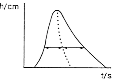
5.50 Elution peak due to diffusion 68
CHAPTER 6
to
6.00 Application of the solvation equation^mberlite XADs 71
6.10 Previous work on XAD-16 and XAD-7 80
References 85
CHAPTER 7
7.00 Application of the solvation equation to liquid polymeric phases 86
7.10 Solid support 86
7.20 Results for uncoated Chromosorb GAW-DMCS, 40-60 mesh size 93
7.30 Correction for logVc for solute adsorption on support 95
7.40 Polymeric phases 97
7.41 Fluoroelastomers 98
7.411 1,1 -Difluoroethene-hexafluoropropylene copolymer and 98
1,1 -Difluoroethene-hexafluoropropylene-tetrafluoroethylene terpolymer
7.412 Tetrafluoroethylene-propylene copolymer 111
7.420 Butyl rubbers 121
7.430 Ethylene-propylene copolymers 133
References 139
CHAPTER 8
8.00 Application to SAW chemical sensor 142
8.10 Background to SAW devices 142
8.20 Selection of coating material, physical properties 148
8.30 SAW device used in sensor array 150
8.40 Characterisation of polymeric candidate SAW phases 155
8.50 The regression equations of the polymeric phase 156
8.60 Summary of the polymeric candidate phases 171
8.70 The grouping of characterised phases 175
8.80 Characterisation of candidate solid phase for SAW sensor 180
9.00
CH A PTER 9
Solvatochromism of solvent and polymer 206
9.10 Effect of solvent on ultra-violet/visible absorption spectra 206
9.20 Solvatochromie comparison method 209
9.21 Solvent dipolarity/polarisability, 7t*i 21 0
9.22 Solvent hydrogen-bond basicity, p, 21 2
9.23 Solvent hydrogen-bond basicity, ai 214
9.30 Previous work on solvatochromism with polymers 218
9.40 Result and discussion on solvatochromie data 219
9.50 Determination of fragment parameters 230
9.60 Analysis of the solubility of fullerene in various solvents 233
9.61 Ruoff et al solubility data 234
9.62 Mathews and co-workers solubility data at 303K 237
9.70 Experimental procedures 247
9.71 Procedure for solvatochromie measurements of solvent 247
9.72 Procedure for solvatochromie measurements of polymer films 248
References 250
10.00
CH A PTER 10
Summary discussion and future work 252
11.0
CH A PTER 11
Experimental: liquid phase 255
11.10 Measurement of relative partition coefficients 255 11.20 Measurement of absolute partitition coefficient 255
11.30 Experimental details 256
11.31 Preparation of gas-chromatographic column 256
11.32 Packing of a column 257
11.33 Column length 259
11.34 Conditioning of a column 259
11.35 Operation procedure 259
11.40 Experimental: solid phase 261
11.41 Column packing and conditioning 261
11.42 Column length 262
11.43 Operation procedure 262
11.44 Data collection 262
ACKNOWLEDGEMENTS
I owe my depth of gratitude to my supervisor Dr. Michael Abraham, whose unfailing encouragement and sound advice over the past four years has been pivotal in the accomplishment of my research. It is impossible to imagine life as a student without this level of support and understanding. Thank you.
I also like to thank the teams of past and present; Dr. Jenik Nazari-Dehnavi for the advice of inverse gas-chromatography when I was new to the area, and for the many other discussions on various matters. Dr. David Walsh who imparted his knowledge on the ‘ins and outs’ of adsorbent work. Dr. Harpreet Chadha for encouraging me to ‘get in-to’ computer, and Dr. Andy McGill for the advice on solvatochromie work.
All the best to Juliet Osei-Owusu who has been a constant and supportive companion and good luck to Julian Dixon and Vikas Gupta in their present work.
I would like to thank Dr. Wendel Shuely for his guidance and support and contribution to my knowledge of the technical aspects of the polymer materials. I am also grateful for his proof reading of my work. And to Dr. Jay Grate for his help and advice.
I cannot fail to thank the technical staff from workshops in the Chemistry Department, Dave Knapp, Jo Nolan, Dick Waymark and Sam Gardiner, who have been an enormous help. I would also like to extend my gratitude to Leslie Spencer, Frank Barretto, who were always willing to help, and Kelvin Reeves for the guidance on SEM.
Last but not least I greatly appreciate my family whose understanding and support has been without bounds, to whom this Thesis is dedicated. My friends for tiredlessly lending their ears and being readily available when help is needed, in particular Dorothy Kamya and Paulomi Shah.
Thank you to David Venezky for funds to purchase fullerene, and to the the US Army and to the US Navy for support, enabling this work to be carried out.
CHAPTER 1
1.00 Introduction to chromatography
One of the notable scientific achievements of this century is the discovery and application of chromatography. The technique was devised by the Russian botanist M. S. TswelT* in 1906, to separate plant pigments by a chromatographic method (now called liquid-solid chromatography). The word chromatography, literally "colour writing" was used by Tswett to describe the process. Progress in the development of chromatography reached a breakthrough in 1941 by Martin and Synge^ in partition chromatography for liquid-hquid chromatography, followed by the invention of gas-liquid chromatography in 1952 by James and Martin,^ based on the differences in partition of separated substances between the gas phase and a hquid phase.
Chromatography can be considered as a science of analysis and preparative separation of substances, or as a method of studying physicochemical properties."^ The feature common to all chromatographic methods is the use of two phases, one stationary and the other mobile; separations depend on the relative movement of these two phases. Chromatographic methods may be classified according to the nature of the stationary phase, which may be a solid or a hquid. If the stationary phase is a solid the method is known as adsorption chromatography; if a liquid, as partition chromatography. In each case the mobile phase may either be a liquid or a gas.
1.10 Gas Chromatography
The gas chromatographic methods that were used in these physicochemical studies were gas-liquid and gas-solid chromatography, and can be summarised as:
the support, while the mobile gas phase flows through the spaces of the solid particles.
- Gas-solid chromatography^ (GSC), when the mobile phase is a gas, the stationary phase is a fine particle or porous solid, providing large area of contact between the two phases.
The first experimental work on gas-liquid chromatography was published by James and Martin.^ Today, literature on chromatography contributes significantly to all kinds of research, from pharmaceutical, agrochemical to polymers. This extensive application includes high performance hquid chromatography (HPLC),
capillary and chiral separation chromatography and many more.
Chromatographic techniques have become classical and their use is without doubt diverse, powerful and an indispensable tool in scientific work.
1.20 Chromatographic processes
There are three main ways to operate a chromatograph,^ depending on how the solute is fed into the column.
In elution chromatography, a small discrete volume of sample is introduced into the column and carried by the flowing mobile phase, the different components in the sample are separated according to the distribution coefficient between the two phases, and their emergence at the outlet end is suitably detected.
In displacement chromatography, a displacer is introduced into the mobile phase, the displacer must have a higher affinity for the stationary phase than the sample. The displacer then drives the adsorbed components progressively along the column, each component displacing the one in front, until they are eluted in the same order in which they were adsorbed on the column; the least strongly retained being eluted first.
Displacement chromatography is sometimes used in preparative chromatography and frontal chromatography in some physicochemical measurement applications, but of the two methods, elution chromatography is more commonly used.
1.30 Instrumental components of gas-chromatography
The principle function of a gas chromatograph is to provide conditions required by the column to achieve separation of components carried in the mobile phase, without lowering the performance of the column. The gas-chromatograph consists of a regulator by which the flow of carrier gas into the column is controlled, an inlet system to vaporise and mix the sample with the carrier gas, a thermostated oven and an on hne detector to monitor the separation. Instruments differ in their degree of sophistication and degree of tolerance within which the experimental conditions can be controlled, but the basic components are the same, see figure 1.0
1.31 Pneumatic system
CR
FÇ
PR
AC
DC
He
GC
Key: FC Flow Controller
I
Injection Port
M Manometer
AC Adsorbent Column
FED Flame Ionisation Detector
A Amplifier
CR Chart Recorder
A/D Analog Digital Converter
C Computer
GC Gas Cylinders and Pressure Regulators
DC Drying Column
PR Pressure Regulator
but this has a negligible effect on the solute partition coefficient. The solubility of the carrier need only be considered when the gas-phase interactions are measured by varying the total pressure.
The carrier gas is supplied from a pressurised cylinder at high pressure, which is coarsely controlled by a pressure reducing valve at the outlet. A steadier flow of gas to the instrument is controlled by a second regulator, this fine flow tuning is positioned before the gas entes the control. The carrier gas first is purified by directing the gas flow through a molecular sieve trap to remove oxygen, low molecular weight hydrocarbon and moisture. Oxygen present in the carrier gas causes degradation of the stationary phase and shortens the life span of thermal conductivity detectors. While moisture can also cause the above effect, it is also a strong deactivating agent, which results in poor reproducibility of retention times in gas-solid chromatography.*
The flow of the hydrogen and air gases required for flame detectors need only be coarsely controlled. Usually, a pressure regulator at the head of the gas cylinders is
.coupled with a needle valve. The flow control of carrier gas is more precise, as variation of gas flow affects the retention reproducibility.
1.32 Injector system
The start of analysis begins when a liquid or gaseous sample is injected into the injector port, purposely designed to be near to the head of column inlet to avoid diffusion of sample in the gaseous phase. Liquid or gaseous samples are usually injected using a microsyringe through a silicone rubber septum, which is resistant to high temperature, and sealable to prevent the escape of the vapours. The injected sample, if a liquid, is vaporised rapidly in the injector port to prevent band broadening, tailing and prolongation of retention time.^ The vapo rised sample is led to the start of the column by the carrier gas. The injector temperature is set based on the solute molecular weight and requirement for a particular analysis.
1.33 Sample size
The size of the sample required depends on whether the study carried out is in the infinite dilution range or in the range of finite concentration for gas-liquid chromatography and gas-solid chromatography techniques. At infinite dilution, the concentration of the sample is negligible and thus the gaseous phase may be considered as ideal. The term ideal means that there is no peak broadening, but in most cases non-ideal chromatography often exists. At infinite dilution, the sample molecules do not interact with each other and therefore behave independently, and thus lead to linearity of chromatography, at this region of concentration. With linearity the peaks are symmetrical, with easily defined retention volume and column efficiency measurements. With finite concentration, larger amounts of solute are generally required. The amount sorbed is less than proportional to the concentration in the gas phase, and this leads to peaks with sharp fronts and diffuse tails.
1.34 Column oven
The column ijplaced in the oven with the inlet end connected to the injector port and the outlet to the detector. The column oven is generally a forced circulation air thermostat of sufficient size to accommodate the column. Its functions are to heat the column to the required temperature and to maintain the uniformity of the temperature, because fluctuation of temperature of the column is one of the main causes of peak distortion, affecting the distribution constants of solutes between the mobile and stationary phase, hence the retention times.
1.35 Gas detector
Organic vapors in the effluent from a gas chromatograph can be detected by two main methods: flame ionisation (FID) and thermal conductivity (TCD), these detectors respond to nearly all organic compounds. Detectors can be characterised as mass or concentration dependent, and this feature is observed in the signal of the gas chromatographic detector. A detector is described as concentration-dependent when its sensitivity is dependent upon the flow rate through the detector, ionisation detectors. Sensitivity is thus the product of peak area and flow rate divided by the weight of the sample, see equation 1.0. A detector is mass-dependent when its response is not effected by the gas flow rate, thermal conductivity detector, and sensitivity is defined as the peak area. A, divided by the weight of the sample.
S = F w * A /W (1.0)
Here S is the sensitivity, Fw is the carrier flow rate and W is the weight of the sample. The performance of different detectors are usually considered in terms of minimum quantity standards measurable (sensitivity), the selectivity response ratio between standards of different composition or structure, and the range of the linear portion of the detector-response calibration curve.
construction, low dead volume and fast signal response, and exceptional linear response range.* The disadvantage of FID is its inability to detect certain compounds, such as water, inorganic gases (NH3, SO^), and single carbon bonded to oxygen or sulphur (CO^, SO^). The advantage of non-response of FID to water enables humidity studies to be carried out, however.
The FID functions by burning organic compounds from the column carried in the stream of carrier gas at a small jet hydrogen-air diffusion flame. The resultant ions are concentrated at the collector located a few milhmetres above the Jet flame, and are measured by the difference in the current ion potential between the jet tip and the collector electrode. The potential is selected at the region for which increasing the potential does not increase the ion current ie. the saturation region. The small ion current signal is amplified. Factors that affect the performance of the detector are the ratio of air to hydrogen to carrier gas flow rates, and the sample size. Typical flow rates^ would be: carrier 30 ml/min, hydrogen 40 ml/min (80 ml/min if carrier is helium) and air 500 ml/min. The sample size affectg the detector performance by becoming an additional fuel source to the flame, increasing the flame length. As the flame length increases it penetrates the interior of the collector electrode where the electric field is weaker and the efficiency of the ionisation collector decreases.
caused by the presence of eluted vapour, results in a change in the temperature of the wire, and unbalance of the bridge.
Katharometer is a robust and easily operated instrument. It is necessary to ensure that the filament is never energized when the gas flow is stopped. Otherwise the filament can bum out within a few seconds. On first starting up, sufficient time must be allowed for air to be swept out of the system before the katharometer is switched on, to prevent oxidation of the filament.
For many general applications FID is preferred, it has sensitivity^ of some four to six orders of magnitude ^than that of katharometer, has a greater linear response range, and provides a more reliable signal for quantitation.
1.36 Measurement of retention time (t^)
The method adopted to measure retention time is important as this directly affects the accuracy of chromatographic determinations. Any errors in measurement depend on the method of measurement adopted, and would be relatively greater for substances with a short retention time. The commonest techniques used are:
1. Stop watch (only for very short retention) 2. Electronic integrator
CHAPTER 2
2.00 Theoretical basis for gas chromatography
The normal way of obtaining the result from a gas chromatographic measurement is in the form of a chromatogram. From measurement of the chromatogram, retention volumes or relative retentions may be determined which are characteristic of individual compounds.
2.10 Retention times and retention volumes
A chromatogram is a plot of detector response against time, or against the volume of the carrier gas. The horizontal axis, which is the direction of motion of the chart recorder paper, represents time if the paper moves at a constant rate; it also represents volume of gas if the flow rate is constant. The vertical axis represents the concentration of the solute in the gas for a differential detector and will normally be measured in millivolts, see figure 2.0. On an integrated chromatogram, the vertical axis represents the quantity of substance.
S o lu t e in jec tio n
E lu tio n o f
n o n - s o r b e d s a m p l e
E lu tio n o f s o lu t e p e a k
cn
T im e —
The solute retention time, t^, is the time the average molecule of solute takes to travel the length of the column and is measured to the midpoint of the symmetrical breakthrough curve, figure 2.1. A part, t^, of this time is required by all solutes simply to pass through the mobile phase from inlet to outlet. All molecules spend the same amount of time in the mobile phase during their passage through the column, and part of the time is spent in the mobile phase and part of the time in the stationary phase. The contribution to retention by the stationary phase alone is the adjusted retention time, tR>:
(2.0)
Tangents drawn to ttm inflexion points 1.000
0.882 E
9 E E 0.607 o
0.500
Inflexion points
"o
CL 3<r
X
0.134 0.044
In chromatographic separations, the ratio of the time spent by the solute in the stationary phase to the time it spends in the mobile phase must be optimized. This ratio is called the solute capacity factor and is given the equation 2.1
k — 1r / t m = ( t R - t m ) / t m ( 2 . 1 )
Where k is the capacity factor. To plan a strategy for improving separation, it is often necessary to determine k for one or more bands in the chromatogram. Often, only a rough estimate of k is required, in which case k can be determined by simple inspection of the chromatogram, without exact calculation. From its capacity factor, the retention time of any solute can be calculated from equation 2.2
tR = tm (l+ k) = (L /u )(l+ k ) (2.2)
Here, L is the column length, and u is the average mobile phase velocity.
The relative retention of two adjacent peaks in the chromatogram is described by the separation factor, a , given by equation 2.3
a = t R ’ ( B ) / t R ’ ( A ) = k s / k A (2.3)
By convention, the adjusted retention time or the capacity factor of the later of the two elution peaks is made the numerator in the above equation; the separation factor, consequently, always has values greater than or equal to 1.0. The separation factor is a measure of the selectivity of a chromatographic system, and it sometimes can be called the selectivity factor, selectivity or relative retention.
Retention is usually measured in units of time for convenience. Volume units are also used, and if tj^ and t^ are multiplied by the mobile phase flow rate, F, observed at the pressure at the column outlet, the retention volume, and the mobile phase hold up, V^, are obtained.
The adjusted retention volume, V^’, is:
Vr' = Vr - (2,5)
Under average chromatographic conditions, liquids can be considered incompressible, but not so for gases. In gas chromatography, there is a pressure gradient along the column, and the gas flow rate at all points in the column is less than that at the outlet. The elution volumes, V^, V^' and are measured at outlet pressure, and may be corrected to column pressure by multiplying by a pressure-gradient correction factor, f s , thus giving rise to a corrected retention volume, V \ , defined as:
V°R = FIr (2.6)
and a corrected mobile phase holdup,
Vo„ = J^ * F t„ (2.7)
and a net retention volume.
Vn = ^ 3 * V r
= V °R-V0^
= A ( Vr - v j ( 2 .8 )
It is the net retention volume from which equilibrium thermodynamic parameters are calculated, f s is given by;
= 3 [(? / P J '- 1] / 2 [(? / ?„)’-1 ] (2.9)
actually indicates the pressure drop across the column; thus, the inlet pressure is a combination of pressure measured from the gauge and pressure outlet. The pressure-gradient correction factor, f s , is always equal to, or less than, unity.
The reason is that as the peak migrates it moves progressively faster due to increasing velocity of the gas as it expands; the measured t^ relates to a column-averaged velocity, F^, but is multiplied by the maximum (exit) velocity in calculating Vj^, which accordingly is an over estimate of
The mobile gas flow rate is measured with a soap-film meter, and for accurate measurements it is necessary to correct the measured value of the flow rate for the vapour pressure of the soap solution (assumed to be the same as the vapour pressure of pure water) and also for the difference in temperature between the column, T^, and flow meter, T^, as shown below;
Fc= [ T / T J [ 1 - ( P ^ P J ] (2.10)
Where is the corrected carrier gas flow rate, F^ is the measured gas flow rate at the column outlet, P^ is the outlet pressure and P^ is the saturated vapour pressure of water at T^. In these circumstances becomes;
= jV F,(Vr - V J (2.11)
2.20 Specific and relative retention volumes
Many physicochemical constants can be determined from either the specific retention volume, or the relative retention volume. The specific retention volume, Vq, is characteristic of a particular solute, stationary phase, and carrier gas. It is the net retention volume for unit weight of stationary phase and is given by
Where Wi is the mass of stationary phase in grams present in the column. Vg is experimentally obtained via equation 2.13, from relative retention time, trei, and where all the experimental variables are included;
Vg = t„ ,[F c * J^ /W |] or
Vg = Ui*[F»(P„ - P„)Tc* A / PoTwW,] (2.13)
The variables Fw is the gas flow rate at the column outlet, Po is the outlet pressure, Pj is the pressure inlet, Pw is the vapour pressure of the water at the temperature of the soap-bubble flow, Tw, Tc is the column temperature, Wi, is the weight of the stationary phase on the column, and trei is the relative retention time, trei, is defined as the retention time of the solute divided by the retention of a 'standard' under identical conditions. The relative retention is given by*
trei = - 1^/ tR, - 1^ (2.14)
The relative retention is determined from the chromatogram by measuring the by
distance on the chart between the solute peak and an inert peak, and^dividin^thisby th& same distance for the standard solutes. Commonly, the standard is an n-alkane as these are usually readily available in a pure state and often enable comparison to be made with other work.
The use of relative retention times, where appropiate, has two main advantages over absolute (specific) retention volumes. First, since relative retentions are calculated directly from distances on the chart recorder, no knowledge of inlet or outlet pressures, gas flow rate, or amount of stationary phase is needed. Second, relative retention times are more reproducible than specific retention volumes between various 'runs' and often more reproducible between different workers.
The effects of slight variations of column temperature, stationary phase loading, etc., are minimised because the retentions of both solutes are similarly affected.
The retention volume may be related to a physicochemical property of the solute- solvent system, the partition coefficient, K. This is defined as;
K or L = Concentration of the solute in stationary phase (2.15) Concentration of the solute in mobile phase
The gas-liquid partition coefficient is related to the capacity factor by equation 2.16.
K = pk (2.16)
Where p is the phase ratio and is equal to the ratio of the volume of the gas (Vg) and liquid (Vi) phases in the column. For gas-solid chromatography the phase ratio is given by the volume of the gas phase divided by the surface area of the stationary phase.
The partition coefficient, K or L, is dimensionless. The gas-liquid partition coefficient is evaluated from the specific retention volume using the equation below.
K = Wq/ (2.17)
And substituting equation 2.13 into equation 2.17
K or L = t,ei*[Fw(Po - Pw)T.*A / PoT„W, p,] (2.18)
Where is the liquid phase density at the column temperature, and K is the gas- liquid partition coefficient.
A G = - R T , l n K (2.19)
Where AG is the partial molar Gibbs free energy of solution.
2.30 Factors affecting column efficiency
In an ideal column at infinite dilution, a peak profile of a sample would maintain its initial shape as it migrates across the column, ie. an infinitely narrow injected peak would still be infinitely narrow at the outlet. In real columns; as a sample travels through the chromatographic column its distribution about the zone centre increases in proportion to its migration distance or time in the column. The width of the peak
%
spread ^approximately proportional to the square of distance travelled along the column, and maximum amplitude of the peak falls according to equation 2.20
Cmax- !/(])"" (2.2 0)
The extent of broadening is a measure of performance of chromatographic column. One of the most important characteristics of a chromatographic system is its efficiency or number of theoretical plate n. The plate number n can be defined from the chromatogram of a single peak, usually based on properties of a Gaussian peak profile, see %ure 2.1.
n = a (t^/w)^ (2.2 1)
Where t^ is the retention time, and wj, is the band width (in time units) at half height when a=5.54, w, the peak width at the inflection point when a=4, and wy the peak width at the base when a=16. Thus n is a dimensionless quantity. Alternatively, column efficiency can be measured by the plate height H (also the height of an equivalent theoretical plate or HETP):
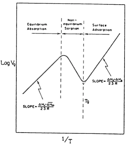
Where L is the length of the column, and H has a length dimension. Column efficiency can also be measured as the number of effective theoretical plates, N, by substituting the adjusted retention time, tR’ for the retention time in equation 2.2 1. The number of effective plates is fundamentally more significant than the number of tVviOfçjUcQL plates since it measures only the band broadening that occurs in the
stationary phase. The two measures of column efficiency are related by equation 2.23
N = n [ k / ( l + k ) r (2.23)
It is good practice, when comparing column efficiency, that n and N should be determined for well retained solutes, because at low k values, for example, k = 1, N will only be 25% of the value of n for weakly retained solutes; however, for solutes that are well retained, k > 10, N and n will be approximately equivalent' ' as shown in figure 2.2. At low k values n will be speciously high and will misrepresent the actual performance. It is^ general practice, to normalise the value of n and N on a per metre of column length basis.
SNoo • 116.9 • 120
100
N_768 200
0.4
The measured quantities n and H are the most useful parameters for characterising the efficiency of a chromatographic system. The names plate number and plate height originate from the plate model of the chromatographic p r o c e s s . H e r e the column is divided into segments (theoretical plates), in which a solute equilibrates rapidly between two phases at each plate before the solute moves on to the next plate. The distribution coefficient of the solute is the same in all plates and is independent of the solute concentration. The mobile phase is assumed to occur in a discontinous manner between plates and diffusion of the solute in the axial direction is negligible. Axial diffusion in chromatography is only insignificant in contribution to band broadening over a narrow range.
The spreading of molecules along the column begins at the injector end of the chromatograph. As the molecules move through the column, the molecules gradually spread out, and this causes the deviation of the average rate process of these molecules. The broadening of the peak shape caused by spreading of the molecules can be separated into two groups. The first involves processes that occur in all columns. These are, spreading due to unevenness of flow (often called Eddy diffusion), longitudinal diffusion, and slow mass transfer in the mobile phase and stationary phase.
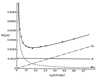
These various contribution to the band broadening can be quantitatively expressed in the van Deemter equation^"^ for HETP;
H = A + B/u + (Cs +Cm)u (2.24)
Where A, B, and Cs, Cm are constants for a given system. These three terms represent plate height contributions from eddy diffusion, longitudinal diffusion, and the sum of stationary and mobile phase mass transfer terms respectively, and u is the mobile phase velocity.
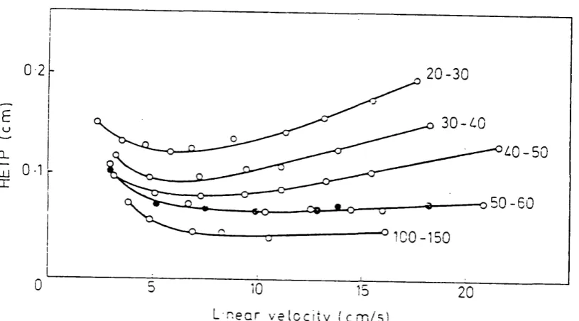
different paths through the packed bed, depending on which flow stream they flbw. This eddy diffusion causes molecules to spread, and this spreading becomes progressively greater as the flow of sample in the mobile phase continues. Band broadening due to this process can be minimised by having the smallest practical particle size with a narrow range distribution,^^ see figure 2.3. A packed column packed with wide range particle size will give rise to band broadening characteristics of the properties of the largest particles while the pressure drop will dictated by the
a(Q,
particles of the smallest size. Both^being detrimental to column performance.
0 2 2 0 - 3 0
0-1
o 5 0 - 6 0
-CQ- o
-0
L n e a r v e l o c i t y ( c m / s
UJ
X
Figure 2.3 Effect of change in the particle size of the support (Silocel)15
ton
Mass transfer is not instanpous in either stationary phase or mobile phases, which are consequently not in complete equilibrium. The result is that the solute concentration profile in the stationary phase is always displaced slightly behind the equilibrium position and the mobile phase profile is similarly slightly in advance of the equilibrium position. The combined peak observed at the column outlet is broadened
tan about its band centre, which is located where it would have been for instanpous equilibrium, provided the degree of nonequilibrium is small.
A minimum plate height is observed at an intermediate "optimum" value of u (u^pj); that is column efficiency is greatest for a flow velocity equal to u^pj, as a plot for plate height and mobile phase velocities indicated.
0 .0 0 6 0 0 .0 0 5 0
0 .0 0 4 0
H(cm)
0 .0 0 3 0
Cu 0 .0 0 2 0
0 .0 0 1 0
B/u
0.1 0.2 0.3 0.6 0.7
References
1. M. Tswett, Ber. Deut. Botan. Ges., 1906, 316.
2. T. Synge and A. J. P. Martin, Biochem. J, 1941, 35, 1358. 3. A. J. P. Martin and A. T. James, Biochem. J., 1952, 50, 679. 4. A. I. Keulmans, Gas Chromatography, 1959, Reinhold, NY. 5. E. Cremer and F. Prior, Z. Electrochem., 1951,55, 66.
6. D. Ambrose, Gas Chromatography, 1971, Butterworths, London. 7. J. R. Conder and C. L. Young, Physicochemical Measurement by Gas
Chromatography, 1979, J. W. & Sons, NY.
8. C. F. Poole and S. K. Poole, Chromatography Today, 1991, Elsevier, Amsterdam. 9. J. G. Litt and N. Alder, J. Chrom., 1965, 3, 250.
10. A. Levy, J. Sci. Instr, 1964, 41, 449.
11. J. Krupcik, J. Garaj, G. Guichon, and J. M. Schmitter, Chromatographia, 1981, 14, 501.
12. B. L. Karger, L. R. Snyder and C. Horvath, An Introduction to Separation Science, 1973, Wiley, NY.
13. J. C. Giddings, Dynamics of chromatography, 1965, Dekker, NY.
14. J. J. Van Deemter, F. J. Zuiderweg and Klinkenberg, Chem. Eng. Sci., 1956, 5, 271
15. J. Bohemen and J. H. Purnell, Gas Chromatography, Edited by D. H. Desty, 1958, Butterworths, London.
CHAPTER 3
3.00 Introduction to linear energy relationship
. The relationship between organic reaction rate coefficients and equilibrium constants and their physico-chemical properties in solution have qualitatively often been siudied-, but quantitatively their understanding for a long time was not so clear. This prompted a need to find an explanation whereby one body of results can be related to another, and thus to obtain quantitative estimates of the factors underlying reactivity. Such a relationship is found in many empirical correlations, in the form of a linear relationship between the logarithms of the rate coefficients (k) or equilibrium constants (K) for one reaction and those for a second reaction subjected to the same variations of reactant structure or reaction conditions. These correlations are appropriately called linear free energy, because at constant temperature logk is related to the free energy of activation and logK is related to the standard free energy change, although ‘correlation equation’ is sometimes preferred. The basic relationships are associated with the name Hammett' (1937), but LFERs hav&been reported earlier. When applied to solvation processes, LFERs are sometimes denoted as linear solvation energy relationships, or LSERs.
3.10 Linear Solvation Energy Relationship (LSER)
The linear solvation energy relationship is based on a simple solvation model used by Abraham, Kamlet and Taft (AKT)^’^ on the concept of a solution of a gaseous solute into a solvent, see figure 3.0. The process can be broken down as follows;
1. The creation of a cavity of a suitable size in the solvent, this involves the endoergic breaking of solvent-solvent bonds
2. The reorganisation of the solvent around the cavity
S o l u t e
S o lv e n t
S o lu t e
S o lv e n t
S olu te S olvent C om plex
w .
F ig u re 3 .0 0 T h e so lv a tio n m o d el
T h e e n d o e rg ic e ffe c ts in m a k in g a c a v ity d e p e n d o n the fo rc e s h o ld in g th e so lv e n t
m o le c u le s to g e th e r, a n d on the size o f the c a v ity . T h is is m e a su re d by th e H ild e b ra n d
c o h e siv e e n e rg y d e n s i t y , e q u a t i o n 3.0. T h e e n e rg y in v o lv e d in re o rg a n isin g the
s o lv e n t m o le c u le s a ro u n d is negli g ib le, e x c e p t fo r a ss o c ia te d so lv en ts.
= (A H -R T )/ V | (3.0)
W ith th e in tro d u c tio n o f the so lu te into th e c a v ity in step 3, v a rio u s s o lu te -so lv e n t
in te ra c tio n s c a n tak e p la c e , all o f w h ic h are e x o e rg ic . F o r a so lv e n t a n d so lu te o f
p o la r o r p o la ris a b le n atu re , d ip o la r in te ra c tio n c a n be set up, Tt*, o f th e ty p e d ip o le -
d ip o le , d ip o le -in d u c e d d ip o le , w ith tc*i fro m the s o lv e n t an d 71*2 c o n trib u te d fro m
the so lu te . T h e c o m b in e d te rm 7i*i7i*2 re p re se n ts th e p o la r in te ra c tio n . H y d ro g e n -
b o n d a c id /b a se in te ra c tio n s can be set up if the s o lv e n t is a h y d ro g e n -b o n d acid, (X|,
acid. This interaction is termed, 0Cip2 or Pitt2 respectively.* If neither the solvent nor the solute is dipolar or acidic/basic, then only general dispersion interaction takes place.
A general equation can be formulated that reflects the various interactions that occur in solubility or solubility related process, SP.
SP = SP„ + Atc*,jc*2+ Ba,.p2+ Cp,.a2 + D(Ôh^), V, (3.1)
Where SP^ is a constant, while the constants A, B, C and D depend upon the solvent or solute property being modelled.
For the solubility property of a single solute in a series of solvents, 71*2, P2, and will be constant and can be subsumed together with the constants. A, B, C and D, giving the equation coefficients s, a, b and h. These coefficients can be obtained by the method of multiple linear regression anal}is (MLRA). Equation 3.1 can then be rewritten as;
SP = S P q + S7t 1 + aoti + bPi + h(ÔH^), (3.2)
Alternatively, for the solubility property of a series of solutes modelled in a given solvent, then the solvent parameters can be taken as constant, ie. 7t i , a i. Pi and (Ôh^),, and the general equation 3.1 can be written as;
SP = SPq + S7Ü 2 + aoc2 + bP2 + mVj (3.3)
nonpolyhalogenated aliphatics compounds, 0.5 for polyhalogenated ones, and 1.0 for aromatics. Equation 3.2 and 3.3 become;
SP = S„ + d.S, + S jt* , + a a i + b p , + h(S^H), (3.4)
SP = Sq + d .6 2 + S7l 2 + a o t2 + b p 2 + mVj (3.5)
In equation 3.5, Kamlet et al have taken the cavity term for a series of solutes in the same solvent as being proportional to either the intrinsic volume, Vj, of Leahy,® or the characteristic volume of McGowan.^ This works well when SP is a liquid-liquid partition coefficient, but for the sorption process of gaseous solutes in liquids or solids, a new parameter was devised, denoted logL'®, where L ® is the Oswald solubiltiy coefficient* on n-hexadecane at 298.15K. The solute volume term is replaced by logL'®;
SP — Sq + d.Ô2 + S7Ü 2 + a(X2 + bP2 + 1 logL (3.6)
The various interactions that take place between solute-solvent are formulated in the equation (solute dipolarity, hydrogen-bond acidity and basicity, and solute size/dispersion).
The general equation 3.5 was revised further by replacing the term d.Ô2 with rR^, where is the solute polarisabiltity, providing a quantitative measure of the ability of a solute to interact with solvent through n and k electrons.^ Similarly, new
dipolarity/polarisability sTt"^ hydrogen-bond acidity aZa"^ and hydrogen-bond basicity bZp"^ parameters were developed by Abraham et al'"'''"'^ to overcome some of the difficulties encountered with the earlier Kamlet and Taft*^ ''* hydrogen-bond scales (a ^ and P J, as shall be discussed further on. However, the use of new
hydrogen bond scales does not negate the old ones, as the scales are very similar and scaled to the same range of zero to one. The new general solvation equation is shown in equation 3.7.
3.20 The general solvation equation; solutes parameters
In carrying out a multi linear regression analyis using the LSER equation, whether it be the solvent equation 3.7 or the solute equation 3.4 requires a knowledge of the relevant parameters or descriptors. The parameters of either solute or solvent need to be identified. The solute parameters were determined by Abraham et al using various methods, and details of how they are obtained are covered next. How solvent descriptors are found will be discussed in a later chapter.
3.21 General dispersion interaction
When a solute enters into a solution, a cavity is formed. The hole is created by first breaking solvent-solvent bonds; this endoergic process is co u n tered by the formation of solute-solvent interactions when the solute sits in the cavity of the solvent. Thus, the size of the cavity can be considered as the molar volume of the molecule at 298 K, V^.
Another parameter, logL’^ was formulated to provide a measure of both cavity size and solute-solvent dispersion interactions. LogL'^ is defined as log of the Oswald solubility coefficient, L on n-hexadecane at 298.15 K, which is identical to the gas- liquid partition coefficient, K. Values of L'^ or K’^ were measured by the method of inverse GLC.
L' ^ o r K‘^= Concentration of the solute in hexadecane (3.8)
Concentration of the solute in the mobile phase
Note that the negative calculated term indicated in the cavity term opposes dissolution of solute in n-hexadecane, while dipersion interaction of solute is favourable. The dispersion interaction is nearly always greater than the cavity term.
3.22 Solute hydrogen-bond acid scale,
The original hydrogen-bond acidity, a^, and basicity scale, were intended only as interim s c a l e s . N e w scales, and were set up by Abraham et al based purely on a thermodynamic basis." The hydrogen bond acidity scale WQS formulated from logK, equilibrium constants of 1:1 complexation of a series of monomeric acids against a given reference base in an inert solvent, tetrachloromethane. Both the acid and the base must be present at low concentration in order for both to be in solution as monomeric and unassociated forms.
A-H 4- B ---► A-H—B
The general scale of hydrogen-bond acidity was set up by plotting a series of acid logK (against reference base) versus a series of logK (against any other reference base), yielded straight lines, with an intersection point at logK = -1.1 (equilibrium constant expressed in molar concentration units). The various logK plots must show family-independent behaviour, so that it is possible to obtain an 'average' hydrogen- bond acidity (with some exception) for solutes in CCl^, denoted as lo g K \. These were then transformed into a hydrogen-bond acidity scale, simply via equation 3.9.
a "2= (logK". + 1.1)/4.636 (3.9)
be practically obtained from complexation constant. Multiple hydrogen-bonding with several solvent molecules gives higher Z a^2 value than could be obtained from a complexation constant, as shown in table 3.0 for the case of solute water.
Table 3.0 A comparison of and Z a"; for some solutes.
Solute I a", Za",
Butanone 1 0.00 0.00
Ethanol 1 0.33 0.37
Pyrrole 1 0.41 0.41
Water 1 0.35 0.82
Acetic acid 1 0.55 0.61
Phenol 1 0.60 0.60
3.23 Solute hydrogen-bond basic scale,
The solute basicity parameter p% was originally taken as identical to pi, the solvatochromie parameter, for non-associated liquids,**’*^ it being thought that a 'monomeric' solute parameter could not be the same as Pi for associated liquids such as alcohols. A new p2 scale was established by Abraham et al, used 1:1 hydrogen- bond complexation constants in tetrachloromethane, P"2- Hydrogen-bond basicity was set up by plotting logK values of a series of bases (against a given reference acid) versus a series of bases (against other acids). These plots gave straight lines passing through some magic point, logK = -1.1, and enabled the average hydrogen- bond basicity, logK% for solutes in CCl^ to be obtained. These values were then transformed into the p^2 scale by applying equation 3.10
The factor 4.636 was chosen so that ^"2 = 100 for the hydrogen-bond base hexamethylphosphortriamide, and has no physical significance other than to serve as a convenient working range of and values.
Just as for the acidity term, there is no certainty that is the appropiate scale to use when a solute is surrounded by the solvent species. However, with a few exceptions can be used as for mono-bases. In the case of poly-base, again there seems to be no alternative than to calculate by back-calculation. Table 3.1 shows a comparison of and values for some solutes
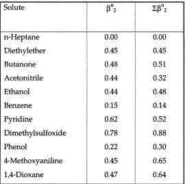
Table 3.1 A comparison of and values
Solute
1 ZP"2
n-Heptane 1 0.00 0.00
Diethylether 1 0.45 0.45
Butanone 1 0.48 0.51
Acetonitrile 1 0.44 0.32
Ethanol 1 0.44 0.48
Benzene 1 0.15
j 0.14
Pyridine 1 0.62
1 0.52
Dimethylsulfoxide 1 0.78 0.88
Phenol 1 0.22 0.30
4-Methoxyaniline 1 0.45
1 0.65
1,4-Dioxane 1 0.47
3.24 Interaction between
n
and n-electron pairThe concept of polarisability is well established , but its quantification was not too easily obtained. The polarisabilty-correction parameter, Ô2, in the LSER is only an empirical factor, limited to one of three values; 1.0 for aromatic compounds, 0.5 for halogenated aliphatics and 0.0 for all other compounds. A number of possible replacements for Ô2 was considered by Abraham et al., molar refraction, MR, being one, as it is often used as a measure of polarisabiltiy. Molar refraction can be defined as;
MR^= 1 0[(n-l)/ (n+2)]V^ (3.11)
Where n is the refractive index taken at 293K with the sodium-D line, and is the McGowan's characteristic volume^* in (cm^mol ')/100. This proves to be of little use, because of the presence of the volume term in molar refraction, the latter always increases with increasing size. The refractive function itself is an indication of the polarisable electrons for a molecule that is either aromatic or a halogenated aliphatic compounds. However, solutes with molar refraction in ‘excess’ of molar refraction^ to an alkane of the same characteristic volume, is defined as R^;
R^ = MR^(observed) - MR^(for alkane of the same V^) (3.12)
The value of MR^ for an alkane of the same characteristic volume is subtracted out, this is to remove the dispersive part already accounted for in logL'^ R^ provides a quantitative indication of polarisable n and k electrons, and is obtainable via
equation 3.11-3.12, once the refractive index, f(n) and for any solute is known. Note, by definition R^ = 0 for all alkanes, and by calculation R^ is also zero for branched chain alkanes and for the rare gases as well. Like MR^, R^ is almost an additive quantity, and can reasonably easy be estimated for solid compounds, although in many cases experimental molar refractions are available. After incorporation of ^ new parameter, the linear regression now becomes;
The term rR^ in the above equation is a quantitative measure of the ability of a solute to interact with the solvent through solute Tt(mainly)- or n-electron pairs.
3.25 Solute dipolarity/polarisability scale, tc^ 2
Originally 71*2 was taken to be identical as to the Kamlet and Taft^^^^ solvatochromie parameter 7C*i for non-associated liquids only. As 7t*i can only be experimentally obtained for liquids at 298.15K, values of k*2 had to be estimated for all associated
compounds (including acids, alcohols, phenols and amides) and solids and gases. In addition, there is present an inherent assumption that 7i*i is identical to 71*2 for non- associated liquid, whilst this may be possible, there might be a few exceptions to the rule. It seemed necessary to set up a scale of solute dipolarity-polarisability based on some experimental procedure that in principle could include all types of molecules. Abraham et al constructed the new dipolar-polarisability parameter, k^2 for use in
LSER from the extensive sets of retention GLC data of McReynolds^'^ and Patte et al.^^ McReynolds measured the specific retention volume, logVo, for several hundreds of solutes on 77 stationary phases. From these data, Abraham et al determined LSER of the type shown in equation 3.13 for each of the phases and found that of the total 75 phases contained no hydrogen-bond acidity at all. Thus the LSER equation is simplified to;
LogV"c = c + rR^ 4- s71*2 + aa"z + 1 LogL'^ 1^)
There are a series of equations (n=l-75), one for each stationary phase, where the constants, c, r, s, a and 1 have been determined by multiple linear regression analysis, MLRA, using known values of the solute parameters, R^, 71*2, Za"2, LogL’^ for as many solutes as possible. Typically, around 150 solutes were included in each regression equation 3.14, generalised as;
The constant was subsummed into the dependent variables to give 75 equations (one for each phase) :
V n - l — r n - l R2 + S n - l 7 t 2 + 2 + l n - 1 L o g L
(3.16) V n -75 = r 11-75R2 + S n-75^ 2 + ^ n -7 5 0 t” 2 + 1 n-75 L o g L * ^
Where
V. = l o g n « - c . (3.17)
The matrix in equation 3.16 can be used in a vertical format, by regarding for a given solute as the dependent variable and the constants r^, s^, a^, and 1^, as four explanatory variables. The unknown coefficients to be calculated by MLRA in the new (vertical) MLR equation^R^, k*2, and logL'® for the particular solute. The
input data now related purely to properties of the solute, n* 2 can be replaced with an
experimentally determined parameter, k ^2
-V(solute) = Vn = R^ r n 4- Sn + a ”2 a„ + LogL'® 1 „ (3.18)
The regression equation 3.18 was carried out, forcing it to pass through the origin, obtaining reasonable values of R^, 71^2, a"2 , and logL'® for the various solutes studied. As R^ is either known or can easily be calculated for any solute, the number of explanatory variables can be reduced by incorporating R^ into the dependent variable:
LogV°o(„) - Cn - r„R2 = V’ = 71^2 Sn + a ”2a„ + LogL'® 1„ (3.19)
The 71^2 are effective n^2 values for a situation in which a solute is surrounded by an
excess of solvent molecules, and so may be more correctly denoted as Ejt":.
These new experimentally obtained parameters are averages for a whole range of stationary phases Further extension to other solutes was carried out using the Patte et al retention data on five stationary phases having no hydrogen-bond acidity. Again, by method of MLRA the coefficients for the five phases were obtained, namely, s, a and 1. This time five values of k^2 were determined by back calculation using
known values of 7t"2, and logL'^ for each solute, which were then averaged.
Although the combination of solutes in the McReynolds and Patte el al sets amounted to several hundreds, there are more solutes not yet accounted for. The above sets missed out simple functionally substitituted aromatic solutes, polyhalogenated aliphatic solutes, nitroalkanes and nitriles.
The aromatic solutes' Tt": values were determined by back calculation using the general solvation equation on Fellous et af^ retention data for seventeen stationary phases. And the values for halogenated or polyhalogenated solutes were again obtained by back calculation using the general equation from retention data on various stationary phases.
The experimentally 71^2 values comprised quite an extensive list, but more can be added. Abraham et al have devised two simple rules governing 7:^2 values for aliphatic solutes:
Rule 1. In any homologous series of functionally substituted aliphatic compounds, 71^2 is constant except for the first one or two members.
Rule 1 would be extremely valuable in the estimation of Tt": values, because if 71^2 was known for a few members of a homologous series, the same value could be applied to all other members, and rule 1 seems to agree to various homologous series Abraham et al have considered.
Rule 2 is not so well founded, as there may be exceptions or amendments to the rule. However, for the moment, rule 2 does seem to allow a very large number of n^2
values to be estimated for aliphatic compounds. It is to be noted that the starting point for application to the rule is not always the simplest member of any series.
3.30 Summary of solute parameters
Rj This is solute polarizability parameter; it provides a quantitative measure of the ability of a solute to interact with a solvent through n and k electron pairs.
71^2 This is solute dipolar/polarisability parameter which measures the solute’s ability to stabi lise a charge or dipole.
Z a"2 This is solute hydrogen bond acidity summation parameter.
Zp”2 Solute hydrogen bond basicity summation parameter
3.40 Correlation and Regression analysis
The theme of the work here is to find a model to correlate the various interactions between the solute and solvent with the known solute descriptors. The general solvation equation 3.7 corresponds to the various processes and interactions between solute and solvent that are possible in the dissolution of a gaseous solute.
With the necessary descriptors for use in the LSER equation found, a method needs to be set up to generate the coefficients in the equation, and the method used is multiple linear regression analysis, MLRA. This is a common technique in statistics, and is an extension of a simple linear correlation, where a series of dependent y values may be linearly related to the independent variable x.
For simplicity, a relationship between two variables is shown, and if it is linear when X values are plotted against y values, then a straight line can be drawn through
the points, and the equation can be written as;
y = mx + c (3.20)
Where m is the slope of the line and c is the intercept on the y axis, x is the explanatory variable used to determine the dependent value y. If there are scattering points in the plot, then drawing a straight line may not be too obvious, and any line chosen will affect the prediction of y values. In such cases, a method called least squares often is used to decide the best straight line to choose. This works by taken into account all the deviations between observed and estimated value of the variable for a line, squaring them and adding them up.^’ The criterion of least squares is that the best line is the one with the least sum of squared deviation. This is not so difficult when only one variable is present, but complications arise as the number of variables increases, as in the case of the general solvation equation. Of course to undertake the application of least squares method on multiple variables would be horrendous without the aid of a computer, but nowadays that is not a problem.^* This technique assumes that any errors involved would be due to the y values, (which may not be entirely true, as in our case where the explanatory variables are mostly
that shouW
one set of regressions is compared with another, any errors in the explanatory variables would in effect cancel out.)
Correlation gives the association between the variables, but it is the regression that uses the variables to help explain the variation in the dependent variables and thus estimates the parameters of the model, and thus provides a test of the validity of the model and the calculation of the confidence limits of the parameters.^^
Correlation alone cannot measure the success of the relationship between the variables. Other statistical methods are used; the standard deviation of the estimate, sd, the correlation coefficient, r and the F statistic. Standard deviation is the square root of the quantity (sum of squares of deviations of individual results from the mean, divided by one less than the number of results in the set), and is given by
r
-sd = 2 [ ( X j - x ) 2 / n - l j (3.21)
Standard deviation has the same units as the property heing measureJ-It becomes a more reliable expression of precision as n gets larger, so sd is a means of assessing its reliability, and is also used in considering the significance of deviant points. The correlation coefficient gives the measure of suctess of the correlation of the dependent variable y against the independent variable x. Here we are interested in the regression as providing an explanation of results in relation to the numerical range of the data sets, and so a correlation obtained should take into account standard deviation, sd. These considerations are essentially embodied in the correlation coefficient equation, r;
r = [ 1 - s d ' ( n - 2 ) / ( f y n ] " ' (3.22)
to a percentage. Thus when x - 0.90 the regression equation explains about 80% of
the variance. It is very important that the correlation coefficient should be considered in relation to the number of data sets correlated. Correlation coefficient does not give any statistically significance evidence of an association between x and y ie. “could the relationship observed reasonably have occurred due to chance alone?”. Tests can be applied to investigate the significance of the coefficient, and dependent on the assumption made in errors distribution, a test is chosen. Student’s T- test assumes normal distribution of errors. The test is set at a confidence limit, usually at 95%, but can go higher to 99%, depending on the accuracy of the test required. This gives the limit to the range of value accepted at this confident interval.
In multiple linear regression analysis, the T- test is performed on each individual variable to test their significance, as sometimes not all variables are necessary and would be indicated by the level of significance, and so may be removed. Another significanatest, however, as used in MLRA is the F-statistic or the Fisher statistic. This test accounts for the number of variables, v, present and the number of data points, n. The value of F-statistic yielded gives an indication of the quality of the regression, the higher the value F, the better is the regression.
F = r " ( n - v - l ) / ( l - r > (3.23)
Here r is the correlation coefficent, n is the number of data points and v is the degree of freedom, which is (v-1), where v is the number of variables. From the equation, it
to
can be seen that the main factors that contribute^the improvement of the regression are; n and r, because as these two parameters increase, F increases.
3.50 Problems with MLRA
Other factors to take into account are the quality and the quantity of the data used in the regression. The quality of the data here means that in producing a general regression equation, a wide spread of explanatory variables is required. This means that a good range from each variable is appreciated, otherwise the coefficient obtained is not meaningful and statistically significant. As mentioned earlier, the number of data points is important, as this improves the reliability of the correlation. It has been suggested that at least five data points are required per variable.
3.51 Application of MLRA in this work
The use of the LSER equation required the measurement of a series of solute dependent solubility property (log SP) which can then be regressed against a set of explanatory variables for each solute. This yields a characteristic equation with coefficients for r, s, a, b and 1 in the solvation equation. These constants generated characterise the significance of the interactions involved and thus give an indication of the system properties, such as in the separation process. The magnitude of the coefficient is proportional to the solvent-solute interaction that the coefficient parameter refeisto. For some solubility system^, not all of the terms in the equation are necjesary, this is shown by a very small or zero coefficient or a low significant T- test. It must be noted that a large coefficient in the H-bond acidity term aEa"z gives a measure of the solvent H-bond basicity. In some solvents, where the main characteristic interaction is through Tt-bonding, then a large coefficient of s would be expected. In solvents where only dispersion interaction occurs, then only 1 is significant; such an example is n-hexadecane.