Essays on Housing Supply and House Price Volatility

(1)

University of Pennsylvania

ScholarlyCommons

Publicly Accessible Penn Dissertations

Spring 5-16-2011

Essays on Housing Supply and House Price

Volatility

Andrew Paciorek

University of Pennsylvania, paciorek@wharton.upenn.edu

Follow this and additional works at:http://repository.upenn.edu/edissertations

Part of theEconomics Commons

This paper is posted at ScholarlyCommons.http://repository.upenn.edu/edissertations/320

For more information, please contactlibraryrepository@pobox.upenn.edu.

Recommended Citation

Paciorek, Andrew, "Essays on Housing Supply and House Price Volatility" (2011).Publicly Accessible Penn Dissertations. 320.

(2)

Essays on Housing Supply and House Price Volatility

Abstract

A typical U.S. family devotes about a quarter of its annual income and half or more of its net worth to housing. Both the level and volatility of house prices thus have important implications for household behavior and welfare, as well as for the aggregate U.S. economy. Recent research has emphasized the importance of housing supply in determining house prices in different U.S. markets. This dissertation comprises three chapters, each of which focuses on constraints on housing supply, house price volatility, or the link between them.

In Chapter One, I use theory and empirical evidence to understand the impact of supply regulation on price dynamics. My estimates confirm that construction lags and marginal costs play critical and complementary roles in driving up costs on the margin, distorting the elasticity of housing supply and amplifying volatility.

In Chapter Two, I use detailed data on zoning and records of housing transactions in the Boston metropolitan area to estimate the channels by which regulation affects the type and quantity of residential construction. I find that restrictive zoning, particularly large minimum permitted lot sizes, drastically increases the costs of new construction, which leads to fewer, larger houses being built.

In Chapter Three, written jointly with Todd Sinai, we test the hypothesis that owning a home hedges a household against correlated changes in the future cost of housing. We find that the cross-sectional variation in house values subsequent to a move is substantially lower for home owners who moved between more highly covarying cities.

Degree Type Dissertation

Degree Name

Doctor of Philosophy (PhD)

Graduate Group

Managerial Science and Applied Economics

First Advisor Todd Sinai

Keywords

house prices, house price volatility, housing supply, housing investment, zoning, regulation

(3)

ESSAYS ON HOUSING SUPPLY AND HOUSE PRICE VOLATILITY

Andrew Paciorek

A DISSERTATION

in

Real Estate

For the Graduate Group in Managerial Science and Applied Economics

Presented to the Faculties of the University of Pennsylvania

in

Partial Fulfillment of the Requirements for the

Degree of Doctor of Philosophy

2011

Supervisor of Dissertation:

Todd Sinai, Associate Professor of Real Estate and Business and Public Policy

Graduate Group Chair:

Eric Bradlow, K.P. Chao Professor and Professor of Marketing, Statistics, and Education

Dissertation Committee:

Joseph Gyourko, Martin Bucksbaum Professor of Real Estate

Fernando Ferreira, Assistant Professor of Real Estate

(4)

For Kate

Without whom I would not have found the motivation, the will,

(5)

Acknowledgements

I began my graduate studies in 2006 as the only student in the Wharton Real Estate doctoral

program. Any initial misgivings about my unique status were quickly overcome as I met

and came to know the faculty and administrators of the Real Estate Department. It is a

wonderful group of people who, both collectively and individually, never failed to offer

their help or advice whenever I needed it. I would like to take this opportunity to thank a

few of them, as well as some others who helped me along the way.

First, I am deeply grateful to Todd Sinai, who guided me expertly through the lengthy

dissertation process and the job market. He was a constant source of encouragement and

good cheer at the moments when I most needed them. His mentorship will always be

reflected in my best work as an economist.

Despite his many obligations, Joe Gyourko made himself available to me whenever I

needed his wisdom. Thanks to his ability to break down complicated issues quickly and

clearly, a ten-minute conversation with Joe was often more productive than an hour with

anyone else. Indeed, it was in large measure because of one of those conversations that I

chose to attend Wharton in the first place.

In addition to his role on my dissertation committee, Fernando Ferreira served as

coor-dinator of the Real Estate doctoral program — which is to say, me — for much of my tenure

at Wharton. He helped me though the process of selecting courses and made sure that I

(6)

counsel at many important junctures.

Katja Seim provided important technical advice as well as an invaluable perspective

on my work from outside the prism of urban economics. I greatly benefited from our

conversations and appreciated that she always seemed as interested in my life as in my

work.

Other faculty members, including Albert Saiz, Maisy Wong, Jeremy Tobacman and

Alex Gelber, offered valuable advice and friendly smiles at many points. Outside of the

strictly academic realm, Yezta Johnson and Elizabeth Spence were instrumental in helping

me navigate the institutional perils of Wharton and Penn. The department computing team

— which consisted at various points of Brandon Lodriguss, Chris Iwane, Nancy Golumbia

and Michal Figura — went above and beyond the call of duty to assist me with various

technical problems, both major and minor.

While I began with the faculty, it was my fellow students who had the largest impact

on my experience in graduate school. Adam Isen, David Rothschild and Ben Shiller were

along for the entire ride, and I am thankful for their friendship, as well as that of Fred

Blavin, Brent Glover, Ed Herbst, Oliver Levine, Andrew Mulcahy, Mike Punzalan and Rob

Ready. More recently, the new cohort of Applied Economics students, including Anthony

DeFusco, Anita Mukherjee, Dan Sacks and Yiwei Zhang, among others, provided the

en-joyable office camaraderie that I sorely lacked at some earlier points.

Though I never really intended it, many of my choices in life have paralleled those of

my brother Christopher. Had I set out to pick a role model, I could not have done better.

Finally, but most importantly, I thank my parents for their quiet but consistent love and

(7)

ABSTRACT

ESSAYS ON HOUSING SUPPLY AND HOUSE PRICE VOLATILITY

Andrew Paciorek

Supervisor: Todd Sinai, Associate Professor of Real Estate and Business and Public Policy

A typical U.S. family devotes about a quarter of its annual income and half or more of its

net worth to housing. Both the level and volatility of house prices thus have important

im-plications for household behavior and welfare, as well as for the aggregate U.S. economy.

Recent research has emphasized the importance of housing supply in determining house

prices in different U.S. markets. This dissertation comprises three chapters, each of which

focuses on constraints on housing supply, house price volatility, or the link between them.

In Chapter One, I use theory and empirical evidence to understand the impact of supply

regulation on price dynamics. My estimates confirm that construction lags and marginal

costs play critical and complementary roles in driving up costs on the margin, distorting

the elasticity of housing supply and amplifying volatility.

In Chapter Two, I use detailed data on zoning and records of housing transactions in

the Boston metropolitan area to estimate the channels by which regulation affects the type

and quantity of residential construction. I find that restrictive zoning, particularly large

minimum permitted lot sizes, drastically increases the costs of new construction, which

leads to fewer, larger houses being built.

In Chapter Three, written jointly with Todd Sinai, we test the hypothesis that owning

a home hedges a household against correlated changes in the future cost of housing. We

find that the cross-sectional variation in house values subsequent to a move is substantially

(8)

List of Tables

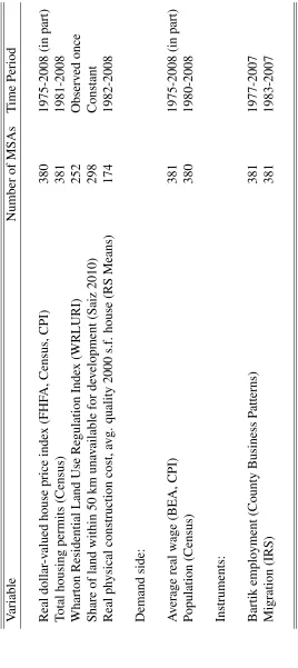
1.1 Data . . . 65

1.2 WRLURI Values for Top 10 MSAs by Population . . . 66

1.3 Myopic Model Elasticity Estimates, OLS . . . 67

1.4 Myopic Model Elasticity Estimates, IV . . . 68

1.5 “First-Stage” Regressions . . . 69

1.6 Structural Model Estimates . . . 70

1.7 Estimated Cost Parameters and Elasticities for Top 10 MSAs by Population 71 1.8 Fixed Costs and Regulation . . . 72

1.9 Robustness Checks . . . 73

1.10 Demand Side (Rent) . . . 74

1.11 Demand Side (User Cost) . . . 75

1.12 Simulation Results . . . 76

2.1 Data . . . 127

2.2 MassGIS Primary Use Codes . . . 128

2.3 Pioneer Insitute Housing Regulation Data . . . 129

2.4 Average Hedonic Results by Year . . . 130

2.5 Lot Size - Zoning Relationship . . . 131

2.6 Variable Costs . . . 133

(12)

2.8 Dynamic Model Estimates . . . 137

2.9 Simulation Results . . . 139

3.1 A Highly Stylized Example . . . 180

3.2 Summary Statistics, By Sample . . . 181

3.3 Baseline Percentage Effect of Covariance on Housing Expenditure Vari-ance . . . 182

3.4 Interacted Percentage Effect of Covariance on Housing Expenditure Vari-ance . . . 183

3.5 Baseline Effect of Covariance on Ex Post Probability of Owning . . . 184

3.6 Interacted Effect of Covariance on Ex Post Probability of Owning . . . 185

(13)

List of Figures

1.1 House Price Comparison . . . 54

1.2 Housing Investment Comparison . . . 55

1.3 Volatility vs. Regulation . . . 56

1.4 Regulation Index Map . . . 57

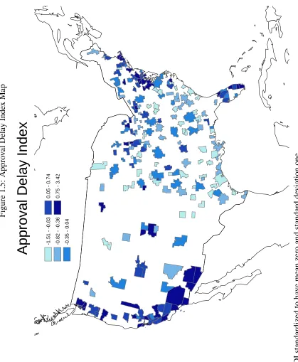
1.5 Approval Delay Index Map . . . 58

1.6 Volatility Map . . . 59

1.7 Housing Demand . . . 60

1.8 Housing Supply . . . 61

1.9 Timeline . . . 62

1.10 Regulation Survey Questions . . . 63

1.11 Impulse Response . . . 64

2.1 Pioneer Institute Data Map . . . 116

2.2 MassGIS Zoning Codes . . . 117

2.3 Price Gradient by Year . . . 118

2.4 Predicted Price by Year . . . 119

2.5 Predicted Price by Tract . . . 120

2.6 Price Gradient by Tract . . . 121

2.7 House Area by Tract . . . 122

(14)

2.9 Flexible Net Price Coefficient Estimate . . . 124

2.10 Net Price Histogram . . . 125

2.11 Net Price by Tract . . . 126

3.1 Covariance Histogram . . . 178

(15)

Chapter 1

(16)

1.1 Introduction

Recent experience in the United States has made painfully clear the importance of housing

market volatility. Housing spending comprises about 25 percent of the median

house-hold’s total income, and housing wealth makes up 55 percent of the median househouse-hold’s

net worth.1 _{Large swings in the price of housing thus have important microeconomic}

ef-fects: Increases benefit homeowners through expansion of paper wealth and relaxed

bor-rowing constraints, while declines tighten those constraints and may leave households

“un-derwater” on their mortgages and unable or unwilling to move. The macro implications

of housing dynamics, meanwhile, are more important today than ever, following a serious

recession and the largest residential real estate boom and bust in at least half a century.

As in most fields of economics, understanding the housing market means understanding

both demand and supply. While the literature on housing demand is voluminous, progress

in understanding the supply side has been much slower (DiPasquale 1999). But recent

con-tributions to the literature on housing supply have emphasized the importance of

construc-tion costs, particularly the costs of complying with zoning and other regulatory constraints,

and the degree to which investment in the housing stock responds to house prices.

In this paper I expand on the existing literature by focusing on the role of regulation and

other supply constraints in amplifying house price volatility, as well as raising price levels.

Intuitively, when supply is unable to keep pace with demand shocks quickly and cheaply,

more of the shocks carry through into prices. In contrast with previous work, I trace out the

channels by which regulation affects the housing market and employ a dynamic structural

model to explicitly estimate the impact of regulation on costs. I find that it is lags and

marginal costs — costs that rise with each additional house built on the margin in a given

year — that explain much of the observable differences in elasticities and volatility across

(17)

markets.

Such differences can be stark, as may be seen in figures 1.1 and 1.2: The median price

of a home in the San Francisco area was about three times as high as in Atlanta between

1990 and 2000. Yet the housing stock of San Francisco grew by an average of just half

a percentage point per year, while that of Atlanta grew by 3.5 percentage points per year.

Moreover, price volatility in San Francisco was far greater than in Atlanta: Even apart

from the trend, the standard deviation of house prices was about twice as high relative to

the mean in San Francisco. Homeowners who purchased in San Francisco thus not only

paid more on average, they faced far greater uncertainty about the capital gain (or loss) they

could expect to realize when they moved to a new house or new city.

Several papers argue that observed differences in construction and house price levels

across metropolitan areas are due to differences in regulation and community opposition

to new construction, rather than shortages of land or higher building costs (Glaeser,

Gy-ourko and Saks 2005a, Quigley and Raphael 2005). Areas with strong demand and tightly

constrained supply experience rising prices and incomes but little construction, becoming

“superstar cities” like San Francisco and Boston (Gyourko, Mayer and Sinai 2006). Other

cities, such as Atlanta and Phoenix, are also in high demand but impose comparatively few

regulations on supply, resulting in substantial expansion of the housing stock and (until

recently) muted price growth.

The strong statistical association between regulation and housing volatility is easy to see

in the data. Figure 1.3 shows a scatter plot and smoothing spline of within-city house price

volatility against the Wharton Residential Land Use Regulatory Index (WRLURI), with

each dot representing a single metropolitan statistical area (MSA).2_{A simple regression of}

price volatility on the regulation measure indicates that a one standard deviation increase

in regulation across cities is associated with about a 30 percent increase in volatility. We

(18)

can get a sense of the geographical nature of this relationship by comparing figures 1.4 and

1.6. In these maps, the darker blue areas, indicating more regulation and higher volatility,

line up quite closely across the figures.

My goal is to use a model of housing supply to explain the causal mechanism

under-lying this relationship. While the empirical literature has convincingly demonstrated that

housing supply conditions can vary widely across regions, housing supply models have

remained mostly ad hoc. Econometric models relating supply to prices and other

funda-mentals have imposed no theoretical structure on these relationships, leading to confusion

even over relatively simple questions such as whether investment should relate to price

lev-els or changes (Mayer and Somerville 2000). Through the careful application of theory to

data on a panel of cities, I make a series of contributions to the literature on housing supply.

Building on preexisting models of investment in durable goods, I develop a dynamic

theory of housing supply that is grounded in the optimization problem of owners of

unde-veloped land. These owners must decide when to build new houses, taking into account

currently available information and their rational expectations about future prices.

Fluc-tuations in prices are driven by demand shocks, such as changes in wages or immigration

patterns. The impact of these shocks on both prices and investment differs depending on

the supply environment, such as the amount of land available, the fixed and marginal costs

of building, and the amount of time needed to build.

My model is explicitly designed so that the parameters can be estimated, and my

pri-mary contribution is empirical. I estimate the structural parameters of the model at the level

of metropolitan areas, using data on house prices and construction, and show how they vary

with observed levels of housing regulation, particularly regulatory permitting and

construc-tion lags. In doing so, I deal with a series of empirical challenges. First, by starting with a

microeconomic optimization problem, I am able to properly specify an estimating equation

(19)

development lags vary across the cities in my sample, I have to carefully model the role of

expectations and their impact on my estimates. Finally, I use demand-side variables that

are plausibly uncorrelated with supply shocks and forecast errors to identify the supply side

parameters.

I find that regulatory costs of all kinds can add tens of thousands of dollars to the

cost of building an additional house on the margin in more regulated cities relative to less

regulated ones. Importantly, while regulations that raise the average cost of new housing or

reduce the amount of available land can lead to higher house prices, it is marginal costs —

which rise with each additional house built in a given year — and construction lags that are

leading causes of volatility.3 Regulatory-induced lags have particularly large effects, both

by adding costs on the margin and by forcing landowners and developers to forecast further

into the future when planning new development, thus lowering the correlation between

actual prices and new supply.

Other authors have not looked closely at how different frictions on the supply side carry

through into observed dynamics. Using the estimated parameters, particular the impact of

supply regulation on costs, I solve and simulate the model to explore the importance of

various constraints. I find that more regulation can significantly increase both the level and

variance of house prices. The model can explain sizable differences in volatility across

metropolitan areas. For example, I predict that price volatility should be about 55 percent

higher in San Francisco than in Atlanta, compared with 100 percent higher in the data.

In the next section I compare my contributions with previous work in the literature. I

then discuss the basics of supply and demand in the housing market before laying out my

dynamic model of housing supply. In Section 1.5 I lay out the data used for estimation,

including the exogenous demand shifters used to identify the supply side. Sections 1.6

3_{Both lags and increasing marginal costs of this kind could result from a variety of types of regulation,}

(20)

through 1.8 detail the precise estimation techniques, use reduced-form regressions and IV

specifications to illustrate the patterns in the data, and then present the structural estimates.

In Section 1.9 I solve and simulate the model to show how the estimated supply parameters

carry through into volatility. The final section discusses caveats and concludes.

1.2 Comparison With Previous Work

Academic work on housing supply has expanded by leaps and bounds since DiPasquale’s

(1999) review of the literature to that date. A series of papers over the last decade have made

clear that constraints on housing supply vary markedly across regions and metropolitan

areas of the United States (Glaeser et al. 2005a, Gyourko et al. 2006, Quigley and Raphael

2005). Differences in supply regulation are crucial for explaining why some cities, such as

New York and San Francisco, have experienced dramatic price growth but relatively little

new construction. Others, such as Atlanta, have expanded their housing stocks substantially

while real prices have risen little.

The impact of these constraints, and regulation in particular, on the dynamics of

hous-ing markets has been explored by few empirical papers. Ushous-ing a metropolitan-level panel

and regressions of housing permits on price changes interacted with regulation variables,

Mayer and Somerville (2000) find that land use regulation lowers the steady state of new

construction and the price elasticity of supply. They also find much more substantial

im-pacts from regulations that lengthen the construction process than from those that simply

add fees or other costs.

While these are important contributions, these papers are reduced-form in nature,

posit-ing simple relationships between price and investment. As DiPasquale (1999) noted, we

still know little about the microeconomics of housing supply, in part because appropriate

(21)

problem, specifically that of the landowner/developer, as in Murphy (2010).4

Unlike Murphy (2010), who estimates cost parameters using microdata from a single

metropolitan area, I focus on observable constraints on the supply side using variation at

the city level. Although the foundation is different, my model leads to a similar investment

equation to that of Topel and Rosen (1988). In contrast with their work, I explicitly

in-corporate land as an input, which has important implications for dynamic optimization; in

particular, investment adjustment costs are not necessary to get forward-looking behavior.

My paper is also closely related to Saiz’s (2010) empirical study of urban growth with

to-pographical constraints on the availability of land, as well as Saks (2008), who examines

the impact on local labor markets of regulatory constraints on housing supply.

Other recent models of housing dynamics include Glaeser and Gyourko (2007) and

Nieuwerburgh and Weill (2009), both of which are spatial equilibrium models in the

tradi-tion of Rosen (1979b) and Roback (1982). Glaeser and Gyourko (2007) establish a series of

stylized facts about the housing market, including that house prices are positively correlated

in the short run and mean-reverting in the longer run, and that both prices and

construc-tion are highly volatile, particularly in inelastically supplied coastal markets. Their model

succeeds in explaining some of the observed patterns, including mean-reversion, but fails

at reproducing others, such as the positive serial correlation of price changes at one- and

three-year intervals.

Using similar data to mine, Huang and Tang (2010) examine the relationship between

supply constraints, including both regulation and land availability, and the sizes of cities’

housing booms and busts from 2000 to 2009. They argue that more constrained cities

expe-rienced larger price run-ups from 2000 to 2006 and larger price declines in the subsequent

4_{The existence of vast new datasets on transactions of new and existing homes offers interesting new}

(22)

period, which generally accords with my findings in this paper. Interestingly, however,

some of the largest price swings in the most recent cycle occurred in relatively

uncon-strained cities like Las Vegas, which is hard to fit with a supply-side explanation alone

(Glaeser, Gyourko and Saiz 2008).

My focus on the initial development decision is related to the real estate applications

of the real options literature, including Grenadier (1996), who looks at overbuilding, and

Bar-Ilan and Strange (1996), who analyze the impact of investment lags on the

relation-ship between investment and uncertainty. A series of papers on land conversion in cities

with stochastic shocks, including Titman (1985) and Capozza and Helsley (1990), examine

the effect of uncertainty on the timing of development and the option value of land. In a

similar vein, Wheaton (1999) provides theoretical support for the important role of supply

constraints, including development lags, in housing cycles. While this literature has

pro-vided useful theory, there are few empirical applications. In one exception, Cunningham

(2007) introduces urban growth controls into a real options model and estimates the impact

of an urban growth boundary around Seattle on price volatility. Finally, while different

in focus and scope, this paper also has links to the real business cycle literature, starting

with Kydland and Prescott (1982), who consider the implications of “time to build” for

macroeconomic fluctuations.

1.3 The Basics of Housing Supply and Demand

Before introducing any notation, it is worth establishing the basics of an equilibrium model

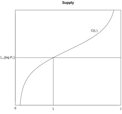
of the housing market via a simple graphical representation. Figures 1.7 and 1.8 show

the demand and supply sides, respectively. In Figure 1.7, a downward-sloping demand

curve relates the implicit rental cost of owning a house in a given period to the quantity of

(23)

thus represented by a vertical line in the figure.

Moving to the supply side in Figure 1.8, we see an upward sloping supply curve relating

the expectation of the next period’s price to the investment that will come online in that

period, under the maintained assumption that it takes one period to build houses. On the

margin, the cost of building an additional house (C(It)) must be equal to the expected

price. As the expected future price rises, investment rises in step. The model is closed by

positing a user cost relation — including interest rates, depreciation, and the full path of

expected future rents — between housing rents and prices, as well as a transition equation

for the capital stock.

An unexpected and permanent increase in demand in period t is represented by an

upward shift in the demand curve. In the short run, supply is fixed, so rents rise. This

pushes the expected future price above the cost of construction. Investment continues until

the price falls back and the system returns to its steady state. When marginal costs are

higher or delays longer, the supply curve is more steeply sloped, so the investment response

is lessened and the return to steady state takes longer. This is the intuition underpinning

my results.

Although there is a time lag in the model, the supply side is myopic in the sense that the

expectation of the next period’s price translates directly into a level of investment, with no

comparison by landowners of expected prices in different periods. Generalizing this world

to a fully dynamic one with forward-looking agents requires explicitly modeling the choice

of when to develop, which I take up in the next section.

1.4 A Dynamic Structural Model of Housing Markets

In formulating a model of housing supply, it is valuable to consider some of the special

(24)

First, a house is not merely durable but extremely so. Although millions of new houses are

built in a typical year, the current bust notwithstanding, the median age of housing units

in the United States is about 35 years.5 Thanks to this durability, housing both provides a

flow of services and serves as a long-term investment, making forward-looking behavior

imperative for home buyers.

Second, the major input into housing is the land on which it is built, which is in fixed

supply within a radius around a given location. This is not to say that there is a shortage

of land in the world. But empty land, frequently on the outskirts of major cities, is poorly

substitutable for land in desirable locations. Landowners thus have some market power,

unlike purveyors of reproducible widgets, and can time their decision to sell or develop the

land. This timing decision forms the core of my dynamic model of housing supply, and it

differentiates my model from most previous approaches in the literature.

Since I employ data on house prices and investment at the metropolitan level, my model

focuses on cities, indexed byj, which I define as infinitely divisible areas of measureAj.

The capital stock of housing inj at timetis denotedKj,t, and new investment isIj,t, with

each period’s capital stock equal to the depreciated last period capital stock plus investment:

Kj,t =Kj,t−1(1−δj) +Ij,t

Each unit of housing takes up one unit of land, so the stock of undeveloped land isAj−Kj,t.

Houses do not differ in quality and are perfectly substitutable.6 The population of the city,

nj,t, is exogenous and evolves deterministically. Endogenizing nj,t would require

model-ing households’ choice among multiple cities, perhaps usmodel-ing a Rosen/Roback-style spatial

5_{2007 American Housing Survey}

6_{The permits data that I use contain no information on housing quality, which is why the model ignores the}

(25)

equilibrium approach, as in Glaeser and Gyourko (2007). Changes in population are an

important source of local housing demand, but for simplicity I incorporate all unexpected

shocks in the demand shockD_j,t.

1.4.1 Demand

Since I focus primarily on modeling and estimating the responses of cities with different

supply constraints to demand shocks, I keep the demand side of the model relatively simple,

in line with the graphical version discussed above and displayed in Figure 1.7. The inverse

demand for housing in cityjat timetis given by

log (Rj,t) =φ+φKlog (Kj,t) +φnlog (nj,t) +Dj,t (1.1)

whereRj,tis the rent paid implicitly by homeowners or explicitly by renters in each period.

WithφKnegative andφnpositive, the amount of housing desired by the exogenously given

populationnj,tis inversely proportional to the rent; that is, the demand curve is

downward-sloping. The demand shock,D

j,t, drives the dynamics of the model.

The price of a house is equal to the present value of current and future rent. Taking

into account property taxes (ωj,t), the mortgage interest rate (rt) and their deductibility

from income taxes (τj,t), as well as a risk premium γ and depreciationδj, we are left with

a standard formula for the user cost of housing (Poterba 1984, Himmelberg, Mayer and

Sinai 2005).7

Rj,t =Pj,t(rt+ωj,t−τj,t(rt+ωj,t) +δj+γj,t−Et[gj,t+1]) (1.2)

HereEt[gj,t+1] denotes the expectation of growth rate in house prices over the next year

7_{Using the mortgage interest rate here implies that houses are entirely financed by debt, with no down}

(26)

taken with respect to all relevant information at timet; in other words, the model relies on

rational expectations. The primary difficulty in calculating the user cost is that expectations

(and the risk premium) are unobserved by the econometrician; one advantage of modeling

housing supply is that it allows me to endogenize expectations in a principled way.

1.4.2 Supply

Owners of undeveloped land, whom I index byi, choose how much land to develop each

period.8 _{I avoid explicitly modeling the market for land or the production function for}

struc-tures by assuming that the construction industry is perfectly competitive, so that

develop-ment risk is borne by the landowner/developer, who also receives any economic profits. In

practice, housing developers buy or option land and undertake much of the risk involved in

the process, but I elide the distinction between developers and original landowners because

my data do not allow me to distinguish between them empirically.

The development and construction of a house inj started att−Lj takesLjperiods and

is irreversible once begun. A building permit must be acquired one year before the house

is finished; this is approximately the amount of time that a single-family building project

takes to go from permit to start to completion, according to data from the Census Bureau.

See Figure 1.9 for a timeline of the process. Upon completion, the landowner/developer

sells it and receives the price of housing at that time (Pj,t) less the fixed labor, materials,

and regulatory costs associated with building the structure (Cj,t). I assume all fixed per unit

costs of construction are paid on completion but are known with certainty at the time the

decision is made.

In addition to the fixed costs, a coherent model requires costs in a given area to increase

on the margin as more investment is undertaken in any period; otherwise all parcel owners

8_{We can extend the model to cover multi-unit dwellings by reinterpreting} _A

j as the total number of

(27)

would want to develop at the same time. Along with construction lags, which I discuss

below, this is one of the two primary channels by which regulation can affect dynamics, in

addition to driving up fixed costs. I incorporate increasing marginal costs by attributing to

each landowner i a random shock to the cost of building χi,j,t−Lj. Since this is the only

parcel-level heterogeneity in the model, I can sort the landowners according to this shock

without loss of generality. Within a given city and time period, these cost shocks follow a

mean-zero cumulative distributionF_j−1 Ij,t

Aj−Kj,t−1

plus an overall mean cost shifterS

j,t.

The scale parameter of this distributionσ_jχvaries across cities, allowing different regulatory

regimes to have disparate impacts on the cost of building on the margin. The mean costS_j,t

affects all landowners inj equally and serves as a city-level supply shock.

The cost of construction may also vary with the amount of undeveloped land that

re-mains available in the city. Costs are likely to increase as the city’s best land is developed,

and the gradient may vary across cities either due to regulatory or topographical constraints

(Saiz 2010).9 _Let_η

j(Kj,t−1, Aj)denote a cost function that depends on the level of the

cap-ital stock relative to the total land area of the city.10

Since construction always takes at least one period, landowners must form expectations

about the path of house prices in order to decide whether to develop a given parcel now or

wait. If a landowner chooses not to build on a given parcel att, she will face precisely the

same choice one period in the future, after receiving any income from the current use of

the land (U¯j,t), such as farming or the operation of a parking lot.

The state space (Sj,t) comprises all information known att, including the evolution of

9_{This sort of variation in costs can also capture a gradient in demand, as in a traditional monocentric city}

model.

10_{Note that I do not incorporate these costs as persistent heterogeneity at the parcel level, which would be}

(28)

the demand shock up to t and the capital stock Lj −1 periods in the future. The future

capital stock up to that point is known with certainty because the investment decisions

have already been made in periods prior to t. In the simplest case, in which the demand

and supply shocks follow first-order Markov processes, the state space contains the capital

stock and current shock realizations:

Sj,t−Lj = n

Kt−1, Dj,t−Lj,

S

j,t−Lj

o

Using the above notation, a landowner’s expected timetvalue from building on parcel

iis

V_j,tB Sj,t−Lj

−χi,j,t−Lj =β

Lj _E_log_P

j,t|Sj,t−Lj

−logCj,t

−ηj(Kj,t−1, Aj)

−S_j,t₋_L_j−χi,j,t−Lj

I specify the price and cost terms in logs because it is an empirical regularity that log

in-vestment increases linearly with log price, whether or not expectations about the future are

taken into account.11 _{Given this, it is unsurprising that most previous research on housing}

supply has specified a log-log relationship between investment and price, and following

that tradition allows for straightforward comparison. Since I have noa priori theoretical

understanding about the cost terms, specifically the functional form ofη(·)or the

distribu-tion ofχ, it is perfectly reasonable to have them relate linearly to log price rather than the

price level.12

Alternatively, the flow value from not building plus the expected value of the option to

11_{I have estimated flexibly nonlinear versions of the model using generalized additive modeling techniques}

(Hastie and Tibshirani 1990, Wood 2006) and do not find substantial departures from the specification de-scribed here.

12_{The concavity of the logarithm also introduces risk aversion, which is reasonable given that the parcel}

(29)

build (or not) tomorrow is

V_j,tN Sj,t−Lj

=βLj_U¯

j,t+βE

max

V_j,tB₊₁−χi,j,t−Lj, V

N

j,t+1 |Sj,t−Lj

There is an equivalence between heterogeneity in fixed costs and in the value of the outside

option, since a higher outside option functions exactly like an increase in the fixed cost of

construction. I attribute all of this heterogeneity to costs, withηj(·)capturing the

increas-ing return from the outside option as land becomes scarce and S

j,t−Lj incorporating any

unobservable shocks to the outside option value.

Since χi,j,t−Lj follows a continuous probability distribution with full support over the

real line and the total land area is divided among infinitely many small parcels, some parcels

will be developed in every city and period. That is, investmentIj,tmust be strictly positive,

so that

Kj,t > Kj,t−1(1−δj)

This is a reasonable requirement for MSAs taken as a whole, since even cities in secular

decline, like Detroit, have new construction in every period.13 Thanks to the lag, each

parcel owner must decide in period t −Lj whether to develop her parcel for delivery at

t. Given the various continuity assumptions, there must be a parcel owner (i∗) who is

precisely indifferent between building and not building. For this owner,

V_j,tB−χi∗_,j,t₋_L

j =V

N j,t

13_{For established neighborhoods, which may see no construction for years at a time, a different formulation}

(30)

or

βLj _E_log_P

j,t|Sj,t−Lj

−logCj,t

−ηj(Kj,t−1, Aj)−χi,j,t−Lj−

S

j,t−Lj

=βLj_U¯

j,t+βE

maxV_j,tB₊₁−χi,j,t+1, Vj,tN+1 |Sj,t−Lj

(1.3)

whereF_j−1 Ij,t

Aj−Kj,t−1

= χi∗_,j,t₋_L

j because the owner is on the margin. This equates the

value of building on the marginal parcel today to the discounted expected value of having

the same choice tomorrow, plus the current income payment.

1.4.3 Empirical Implementation

To estimate Equation 1.3 using a standard panel of MSA-level house prices and

invest-ment — described in detail below — I make a series of additional simplifying

assump-tions, some of which can be relaxed later. First, the discount factor β is known to the

econometrician a priori. Second, the supply shocks S

j,t−Lj are serially uncorrelated, an

assumption that can be tested. Finally, ηj(·) and Fj−1

_I

j,t

Aj−Kj,t−1

have known

func-tional forms. Specifically, I assume that ηj(Kj,t, Aj) = σjη

Kj,t

Aj , which is essentially the

density of housing over a fixed area, and that χi,j,t−Lj

iid

∼ logistic 0, σχ_j, which means

F_j−1

Ij,t

Aj−Kj,t−1

= σ_jχlog

Ij,t Aj−_Kj,t₋₁ 1− Ij,t

Aj−_Kj,t₋₁ !

. Given these assumptions, I can rewrite

Equa-tion 1.3 as follows:

βLj _E_log_P

j,t|Sj,t−Lj

−logCj,t

−ση_jKj,t

Aj

−σ_jχlog

Ij,t

Aj−Kj,t−1

1− Ij,t

Aj−Kj,t−1

!

−S_j,t₋_L_j

=βLj_U¯

j,t+βE

σ_jχlog exp V_i,j,tB ₊₁/σ_jχ+ exp V_i,j,tN ₊₁σχ_j|Sj,t−Lj

(1.4)

where the last term applies the fact thatχi,j,t−Lj+1 follows an iid logistic distribution, so

(31)

To deal with the unobservable value functionV_i,j,tN ₊₁on the right-hand side of Equation

1.4, I employ the representation theorem of Hotz and Miller (1993), who show that value

functions can often be rewritten as functions of conditional choice probabilities (CCPs),

defined as the probabilities that a given alternative is chosen given the state of the world.14

Applying the logistic CDF, we can write the CCP of building next period as

P rB|Sj,t−Lj+1

= exp V

B

i,j,t+1/σ

χ j

exp VB

i,j,t+1/σ

χ j

+ exp VN

i,j,t+1/σ

χ j

Thanks to the assumption that each city has a continuum of identical small

landown-ers, this probability of building is precisely equal to Ij,t+1

Aj−Kj,t, the ratio of parcels actually

developed to the amount of available land. Substituting this into the previous expression,

rearranging and taking the logarithm, we have

log exp V_i,j,tB ₊₁/σ_jχ

+ exp V_i,j,tN ₊₁/σχ_j

=V_i,j,tB ₊₁/σ_jχ−log

Ij,t+1

Aj −Kj,t

I can then plug this expression back into Equation 1.4 and expand theVB_{term to get}

βLj _E_log_P

j,t−βlogPj,t+1|Sj,t−Lj

−(logCj,t−βlogCj,t+1)

−σ_jη

Kj,t−1

Aj

−βKj,t

Aj

−σ_jχ log

Ij,t

Aj−Kj,t−1

1− Ij,t

Aj−Kj,t−1

!

−βE

log

Ij,t+1

Aj−Kj,t

|Sj,t−Lj

!

=βLj_U¯

j,t+Sj,t−Lj

(1.5)

14_{The Hotz and Miller (1993) two-step approach to estimating dynamic models is a popular alternative to}

(32)

where the future supply shock disappears because I assume that the shocks are serially

un-correlated. This is almost exactly the same relation that results from writing the problem of

a single utility-maximizing agent for each MSA and deriving an Euler equation. Intuitively,

this must be the case because there are no cross-parcel spillovers, so maximizing the total

utility of all parcel owners gives the same result as maximizing utility individually, apart

from some minor technical considerations.

There are two remaining complications that prevent estimation of Equation 1.4. The

first is the presence of unobservable expectations, specifically

ElogPj,t−βlogPj,t+1|Sj,t−Lj

. Although I observe the realized prices, I cannot

re-late realizations and expectations without making further assumptions. Following much

of the literature on estimating dynamic models such as this one, I assume that agents

form expectations rationally, so that the equation νj,t−Lj = (logPj,t−βlogPj,t+1) −

Et−Lj[logPj,t−βlogPj,t+1]defines a mean-zero forecast error.

15 _{That is, the subjective}

expectations of landowners are equal to the conditional expectations.

Applying this definition ofνj,t−Lj to Equation 1.5, we get

βLj_((log_P

j,t−βlogPj,t+1)−(logCj,t−βlogCj,t+1))

−σ_jη

Kj,t−1

Aj

−βKj,t

Aj

−σ_jχ log

Ij,t

Aj−Kj,t−1

1− Ij,t

Aj−Kj,t−1

!

−βlog

Ij,t+1

Aj −Kj,t

!

+mj+mt

=S_j,t₋_L_j +νj,t−Lj

(1.6)

15_I _ignore _the _error _in _the _forecast _of _next-period _investment ₍_log Ij,t+1 Aj−Kj,t

−

Ehlog Ij,t+1 Aj−Kj,t

|Sj,t−Lj

i

(33)

Since the outside value of land is not observed, I have foldedβLj_U¯

j,t into Sj,t−Lj. I also

include fixed effectsmj andmtto capture unobservable differences across MSAs and years

in the outside option value and the supply shock. Equation 1.6 comprises only observable

values and explicitly unobservable error terms, which means it can serve as a basis for

estimation, subject to the second remaining complication, that of endogeneity.16

There are at least three possible sources of endogeneity in Equation 1.6: First, the

unobserved supply shockS

j,t−Lj will in general be correlated with realized prices in cityj

at time t, since prices are determined in equilibrium. Second, the forecast error νj,t−Lj is

correlated with the realized valuelogPj,t−βlogPj,t+1 by construction, since the forecast

error is defined to be mean independent of the expectations. Third, the housing stock in

periodt includes investment that comes online in t, leading mechanically to endogeneity

of the housing density term.

Dealing with endogeneity requires a set of exogenous demand shifters that are

corre-lated with the relevant observables but uncorrecorre-lated with both the supply shockS

j,t−Lj and

the forecast errorνj,t−Lj. I discuss my identification strategy after first detailing my data.

1.5 Data

Relative to macroeconomic data, where there is typically one realization of a given time

series, one advantage of researching housing dynamics is that there is substantial

hetero-geneity in housing markets across cities and regions within the United States. Since

supply-side factors like regulation and topography differ widely across metropolitan areas, housing

market heterogeneity allows us to examine the impact of these factors on market

dynam-ics. Essentially, each city is a separate laboratory experiment with different supply- and

demand-side conditions.

16_{In the next section I also specify how I allow the parameter values with}_j_{subscripts to vary across MSAs}

(34)

Table 1.1 summarizes the data used in this paper. I calculate the house price series

using FHFA (n´ee OFHEO) repeat-sales indices deflated by the CPI and pegged to the mean

house price in each city from the 2000 Census. This provides a dollar-valued measure of

prices that controls as best as possible for changes in the types of houses that transact in

any given period.17

I specify new housing investment in each MSA and year using the number of

hous-ing permits issued in that area in the previous year. This lag accounts for the fact that

single-family homes take a bit under a year to complete even after the builder acquires a

permit. I use permits data rather than starts or completions because the Census Bureau has

a detailed inventory of permits that is finely geographically disaggregated. Although it is

possible to abandon permits before starting, and even to abandon units under construction

before completion, Census Bureau estimates indicate that only around two percent of

per-mitted structures are not built, which is not surprising given the substantial costs involved

in preparing for and acquiring a permit. I also use the permits data to calculate the total

stock of housing in each MSA and year by interpolating from decennial census figures.

I focus on the role of three variables that capture supply constraints. The first is the

Wharton Residential Land Use Regulatory Index (WRLURI), which is a measure of

lo-cal regulatory constraints compiled from a 2005 survey of municipal officials (Gyourko,

Saiz and Summers 2008). Figure 1.10 presents example questions from the survey, such

as “What is the current length of time required to complete the review of of residential

projects in your community?”18 _{WRLURI is derived from sub-indices that cover a variety}

17_{The Case-Shiller price indices distributed by Standard & Poor’s, which are the most popular}

alter-native to the FHFA series, do not offer sufficient breadth or length for my purposes. There are 20 MSA-level Case-Shiller indices, which at best go back to only 1987, compared with hundreds of MSAs for the FHFA, many of which start in the early 1980s or before. Although there are some differences between two sets of indices during the most recent boom period, the correlations between the two in-dices over time are still above 0.9 in all metro areas with data from each and above 0.95 in most. See http://www.fhfa.gov/webfiles/1163/OFHEOSPCS12008.pdf for a comparison of the two methodologies.

(35)

of different regulatory constraints, from financial exactions to zoning restrictions to delays

in the approval process. In the context of the model, WRLURI can be interpreted as

af-fecting lags, construction cost, and the amount of available land. That said, Gyourko et al.

(2008) note that the overall index is most highly correlated with the sub-index related to

average delays, which should capture some or all of the regulatory-induced construction

lags. In the empirical work below, I specifically examine the role of the Approval Delay

Index (ADI), which tries to measure the total delay that regulation imposes on the

acquire-ment of a permit.19 _{To complement the ADI, I use a version of WRLURI that strips out the}

ADI as a measure of other sorts of regulation that directly affect costs and land use.

Figures 1.4 and 1.5 map WRLURI and the ADI for every MSA in my sample, with

each color representing one quintile. Table 1.2 shows the WRLURI and ADI values for

the top 10 MSAs by average population over the period from 1984 to 2008, as well as

San Francisco, with both regulation variables standardized to have mean zero and standard

deviation one. The coloration of the map and most of the values displayed in the table

match the standard intuition for which markets are heavily regulated: Coastal cities (San

Francisco, New York) generally display very high levels of regulation by both measures,

while interior cities (Atlanta, Chicago) are typically much less regulated.

The second supply-side variable is a measure of the amount of land in each

metropoli-tan area that is not available for development because it is steeply sloped, with a gradient

greater than 15 percent.20 _{I calculate the amount of developable land in an MSA by}

sub-tracting this measure from the total land area in square miles of each MSA’s component

counties. I further scale this measure by the number of units per square mile in Manhattan,

19_{In practice, the development cycle may be even longer, since getting to the permitting stage may require}

substantial expenditure and years of negotiation with the relevant authorities (Rybczynski 2007).

20_{This is similar to the measure used in Saiz (2010), but for comparability with my other data I calculate the}

(36)

a particularly densely settled area. This ratio of the housing stock to this measure of

devel-opable “slots”, which I refer to as the density of housing, can be thought of as the degree to

which an MSA is currently developed relative to Manhattan.21 If costs rise as metropolitan

areas “fill up”, perhaps because the available land is more expensive to build on or because

the outside option for the land is more valuable, the density should capture this effect.

The last measure is an estimate from the RS Means Company of the real cost of

con-structing a 2000 square foot average-quality house, including labor and materials but

ex-cluding land and regulatory costs (Gyourko and Saiz 2006). The RS Means measure should

translate into an increase in fixed construction costs in the model (Cj,t). The RS Means data

are available in a panel by MSA and year, but WRLURI is observed only once for each

MSA — in 2005, when the survey was conducted — while the Saiz measure is essentially

time-invariant.

1.5.1 Demand Shifters

As in any model of market equilibrium, the quasi-differenced price term in Equation 1.6

is likely to be correlated with the supply shocks precisely because prices are set in

equi-librium. Consistently estimating the supply equation requires one or more variables that

are correlated with house prices and uncorrelated with supply shocks. Given that I allow

the supply parameters to differ across MSAs, these exogenous variables must also provide

variation across both the timetand MSAj dimensions.

To get variation in annual housing demand at the MSA level, I rely on two

plausi-bly exogenous variables. The first (industryj,t) follows Bartik (1991) in using imputed

shifts in local labor demand.22 _{The second (}_migration

j,t) makes novel use of county-level

21_{This is an arbitrary benchmark, but it is convenient and easily conceptualized. In practice there is no}

hard cap on the number of units that can be built in a given MSA; even Manhattan could be built to a much higher density than it currently is without running into a technological capacity constraint (Glaeser, Gyourko and Saks 2005b).

(37)

migration data from the Internal Revenue Service to form an exogenous demand shifter

similar to that of Saiz (2007), who uses “shift-shares” in international immigration patterns

as exogenous local demand shocks in U.S. cities.

To form my Bartik-style labor demand variable I use MSA by industry employment data

from the Census Bureau’s County Business Patterns (CBP).23 Bartik’s (1991) innovation

was to interact national-level shifts in industry-specific employment with the average shares

(across time) of employment or compensation that those industries have in particular cities.

For example, when auto industry employment and/or compensation decreases nationwide

due to a systemic negative demand shock, the city of Detroit and its surrounding MSA

should be particularly negatively affected. To ensure that local conditions in particular

MSAs with sizable shares of total national employment in a given industry do not feed back

intoindustryj,t, I omit cityjfrom the “national” shift in employment when calculating the

variable for cityj.

To provide a useful check on the employment shift-share variable, which is quite

pop-ular in the literature, I also employ county-level migration data from the IRS. The idea

behindmigrationj,t is similar in spirit to that ofindustryj,t: While inflows and outflows

of migrants from MSAjare likely endogenous with respect to local supply shocks, we can

impute overall inflows for MSAj using the other outflows from MSAs that typically send

many migrants toj. For example, outflows from New York to Philadelphia, Washington,

Los Angeles, and other cities change in response to New York-specific shocks. The sum

of these outflows can be used to impute in-migration to Boston, because Boston typically

receives a large share of its in-migrants from New York.

Both variables are exogenous to local supply shocks under reasonable but non-verifiable

house prices and wages. See Saiz (2010), Notowidigdo (2010), Saks (2008), Gallin (2004), and Blanchard and Katz (1992), among many others.

23_{It is also possible to construct an industry shift variable using alternative data, such as paid compensation}

(38)

conditions. Theindustryj,t requires that a city’s housing supply shocks are not

systemat-ically correlated with national industry shocks that differentially affect that city. Similarly,

migrationj,t will be exogenous provided that supply shocks in a given city are not

cor-related with out-migration from other cities that usually send lots of migrants to the first

city.24

1.6 Estimation Strategy

As noted above, least squares estimation of Equation 1.6 would yield inconsistent estimates

for at least three reasons: The market price of housing is determined in equilibrium and is

therefore endogenous, the forecast errorνj,twill be correlated with timetrealizations, and

the lagged housing density int+1is mechanically correlated with shocks to new investment

int.

The first and third endogeneity concerns can be addressed in straightforward fashion: I

use the employment and migration variables detailed in the previous section to instrument

for the house price term, and I use the first lag of of the quasi-differenced density to

instru-ment for the contemporaneous value.25 _{The set of underlying instruments for}_j _at_t_{, which}

I denoteZj,t−1, is thus

Zj,t−1 =

industryj,t−1, migrationj,t−1,

Kj,t−2

Aj

−βKj,t−1

Aj

The employment and migration share variables are strongly correlated, both individually

and jointly, with house prices conditional on the fixed effects; that is, there is a valid first

stage. I explore the strength of the exogenous demand shifters for identifying the structural

24_{As a robustness check, I also estimate the model using a version of the migration variable that includes}

only city pairs that are more than a set distance apart, such as 100 miles. See Section 1.8.4.

25_{Using the lag in this manner requires that the supply shocks be uncorrelated across time, conditional on}

(39)

model parameters in detail in the appendix.

The relationship between the forecast error and endogeneity is more complicated to

address. The standard approach in rational expectations models is to use variables dated at

or before the time the expectations are formed; under the rational expectations assumption

anything in the information set of the agents must be orthogonal to the future forecast

errors. It is neither easy nor desirable to do that in this case, because the true forecast lagLj

differs across cities and may not be perfectly observable, since the Approval Delay Index

component of WRLURI likely only captures differentials in lags caused by regulation,

rather than the overall size of the time needed to plan before building.26 _{Moreover, the effect}

of the forecast error resulting from regulation is not a nuisance in this case but something I

am particularly interested in estimating.

Instead, I adopt a hybrid approach, using Zj,t−1 for prices and investment at period

t. This roughly corresponds with the time at which permits are issued, one year before

construction on a house is completed, which is the bare minimum amount of time needed

for the entire process.27 _{Importantly, however, under the rational expectations assumption}

these instruments will still be correlated with the forecast error betweent−Lj andt−1. To

simplify the notation, letP˙j,t = logPj,t−βlogPj,t+1. Consider the forecast errorνj,t−Lj,

which is defined as above by

νj,t−Lj = ˙Pj,t−Et−Lj h

˙

Pj,t

i

=P˙j,t−Et−1 h

˙

Pj,t

i

−Et−Lj

h ˙

Pj,t

i

−Et−1

h ˙

Pj,t

i

The first term in parentheses in the second line is the forecast error att−1and the second

term is the forecast error between t − Lj and t − 1. Under rational expectations, the

first term is mean independent of information available att−1, since that information is

26_{For example, construction projects in all cities may take an additional year to plan before the city-specific}

approval delay reported in the ADI.

(40)

incorporated into the conditional expectation, while the second term is not. Along with the

mean independence of the instruments from the supply shocks, this implies that

EhS_j,t₋_L

j +νj,t−Lj|Zj,t−1 i

=EhEt−Lj h

˙

Pj,t

i

−Et−1

h ˙

Pj,t

i

|Zj,t−1

i

Rather than making the somewhat implausible assumption that the ADI exactly

mea-sures the total lag, I make the less stringent assumption that

EhEt−Lj h

˙

Pj,t

i

−Et−1

h ˙

Pj,t

i

|mj, mt, Zj,t−1, Dj

i

=α0_j +α1DjE

h ˙

Pj,t|mj, mt, Zj,t−1, Dj

i (1.7)

whereDj denotes the delay index in MSA j. In essence, this assumption means that the

ADI, interacted with realized prices, serves as a proxy variable for the residual forecast

error in Equation 1.7 in the sense of Wooldridge (2002, p. 68). One complication is that

the ADI may not be redundant in the main estimating equation; that is, delays may drive

up costs on the margin as well as increasing the forecast error. Consequently, the ADI term

in the specifications below will capture both the measurement error and true costs, and I

will not be able to separate the two effects without relying on nonlinearities in the moment

condition.

I allow the parameters with j subscripts in Equation 1.3, σχ_j andσ_jη, to vary by MSA

by interacting the primary observables with WRLURI and its sub-indices. Importantly, I

take regulation as exogenously given, rather than allowing it to respond to conditions in

the housing market or even vary over time. This seems reasonable given that I estimate

the model over a relatively short time span, and levels of regulation likely move slowly

over time. This simplification is also necessary, both for data reasons — my measure of

regulation is observed only once for each city — and to keep the model tractable.28 I do,

(41)

however, use preliminary data from a new round of the Wharton survey as a robustness

check; the results are similar to my preferred estimates.

Since I am trying to identify both the main effects and interactions with the WRLURI

indices, I must specify what functions of the exogenous Zj,t−1 and WRLURI I use as the

actual instrument setZˆj,t−1. Following a common practice in the econometric literature, I

run regressions to getLˆ[logPj,t−βlogPj,t+1|mj, mt, Zj,t−1]and

ˆ

LhKj,t−1

Aj −β

Kj,t

Aj |mj, mt, Zj,t−1

i

, the linear projections of the quasi-differenced log price

and housing density onto the fixed effects and the exogenous industry employment,

mi-gration, and lagged density variables. I then multiply these projections by the relevant

components of WRLURI for the specification in question and use the projections and the

interactions as the instruments in a second-step IV procedure.29

The advantage of this approach is that that it is likely to be more efficient than using an

arbitrary set of functions ofZj,t−1 and WRLURI as instruments, since it directly imposes

the interaction in the instrument set. The disadvantage is that, with exactly as many

instru-ments as endogenous variables, I cannot directly test the overidentifying restrictions that

implicitly underly the estimates.

Finally, to estimate Equation 1.6 I must either specify or estimate the discount factorβ.

Identifying the discount rate has proven to be extremely challenging for other researchers,

so I follow much of the literature and simply assume thatβ = .95, a commonly accepted

value.30 _{Even after assuming a value for}_β_{, I must still choose how to deal with the}

com-pound discount factor βLj_{, since I cannot simultaneously identify it with}_σχ

j, σ

η

j, and the

variance of the error term. As I have already argued, assuming values for the construction

lagLj, such as the ADI, is not particularly attractive given that the true magnitude of the

voluminous literature considers its determinants in a theoretical setting. See Calabrese, Epple and Romano (2007) and Fischel (2001) for just two examples of the latter type.

29_{Note the distinction between this and the typically inconsistent “forbidden regression” (Wooldridge 2002,}

pp. 236-237).

(42)

lag may be larger than what is reported, even if the ADI appropriately captures differences

in the lag. Moreover, one of the points of this paper is to study the effects of increasing

the lag. While I must do so indirectly, I certainly do not want to assume away an empirical

question of interest. Instead, I letLj =g(Dj), whereg(·)is a increasing function relating

the ADI to the actual lag. I then divide the entire equation through byβg(Dj)_{and estimate}

the normalized equation.

Applying this normalization and Equation 1.7 to Equation 1.6, specifying the

interac-tions using WRLURI excluding the ADI (W xj) and the ADI (Dj), and taking the

expecta-tion with respect toZˆj,t and the fixed effects yields

E[(logPj,t−βlogPj,t+1)−(logCj,t−βlogCj,t+1)

− σ¯

η₊_σηW x_{W x}

j+σηDDj

βg(Dj)−α1D

j

Kj,t−1

Aj

−βKj,t

Aj

− σ¯

χ₊_σχW x_{W x}

j+σχDDj

βg(Dj)−_α1_D

j

log

Ij,t

Aj−Kj,t−1

1− Ij,t

Aj−Kj,t−1

!

−βlog

Ij,t+1

Aj−Kj,t

!

+mj +mt|Zˆj,t, mj, mt

i

=0

(1.8)

This moment condition could form the basis of an exactly identified nonlinear GMM

estimator with fixed effects. To simplify estimation a bit, take the partial derivative of the

coefficient on the investment term with respect toW xj

∂

¯

σχ₊_σχW x_{W x}

j+σχDDj

βg(Dj)−α1_D

j

∂W xj

= σ

χW x

βg(Dj)−_α1_D

Essays on Housing Supply and House Price Volatility

University of Pennsylvania

ScholarlyCommons

Essays on Housing Supply and House Price

Volatility

Andrew Paciorek

Essays on Housing Supply and House Price Volatility

Acknowledgements

ABSTRACT

Contents

List of Tables

List of Figures

Chapter 1

1.1

Introduction

1.2

Comparison With Previous Work

1.3

The Basics of Housing Supply and Demand

1.4

A Dynamic Structural Model of Housing Markets

1.4.1

Demand

1.4.2

Supply

1.4.3

Empirical Implementation

1.5

Data

1.5.1

Demand Shifters

1.6

Estimation Strategy