R E S E A R C H
Open Access
ApproxMap - a method for mapping blank
nodes in RDF datasets
Juliano de Almeida Monte-Mor
1,2*and Adilson Marques da Cunha
2Abstract
Background: Versioning has proven to be essential in areas like software development or data and knowledge management. For systems or applications making use of documents formatted according to the Resource Description Framework (RDF) standard, it is difficult to calculate the difference between two versions, owing to the presence of blank nodes, also known as bnodes in RDF graphs. These are anonymous nodes that can assume different identifiers between versions. In this case, the challenge lies in finding a mapping between the sets of blank nodes in the two versions while minimizing the operations needed to convert one version into another.
Methods: Within this context, we propose an algorithm, namedApproxMap, for mapping bnodes based on extended concepts of rough set theory, which provides a way to measure the proximity of bnodes and map them with closer approximations. Our heuristic method considers various strategies for reducing both the number of comparisons between blank nodes and the delta between the compared versions. The proposed algorithm has a worst-case time complexity ofO(n2).
Results: ApproxMapshowed satisfactory performance in our groups of experiments, as the algorithm that obtained solutions closest to the optimal values. This algorithm succeeded in finding the optimal delta size in 59% of the tests involving optimal values.ApproxMapachieved a delta size smaller than or equal to those of existing algorithms in at least 95% of the tested cases.
Conclusions: The results show that the proposed algorithm can be successfully applied to versioning RDF documents, such as that produced by software processes with iterative and incremental development. We recommend applyingApproxMapin various situations, particularly those involving similar versions and directly connected bnodes.
Keywords: Blank nodes; Resource Description Framework (RDF); Mapping; Rough set theory
Background
In areas such as software engineering, databases, and Web publishing, methods for versioning have already been developed and successfully applied. These methods must be able to calculate the differences (i.e., deltas) between versions to provide efficient storage of subsequent ver-sions.
Particularly in software engineering, versioning algo-rithms are usually based on a comparison of text lines. However, these methods are not suitable to control
*Correspondence: [email protected]
1Federal University of Itajuba - UNIFEI, Campus of Itabira, Rua Irma Ivone Drumond, 200, Distrito Industrial II, Itabira, MG 35903-087, Brazil
2Brazilian Aeronautics Institute of Technology - ITA, Praca Marechal Eduardo Gomes, 50, Vila das Acacias, Sao Jose dos Campos, SP 12228-900, Brazil
versions of structured or semi-structured documents. In this article, we focus specifically on the version con-trol of documents following a Semantic Web standard, the Resource Description Framework (RDF) [1]. We have applied Semantic Web technologies in the software con-figuration management (SCM) domain [2].
RDF defines a basic data model for writing simple statements about Web objects or resources. It allows the definition of sentences through ‘subject-predicate-object’ triples; that is, a resource, a property, and a value (which can be a literal or a resource). An RDF triple, like a graph’s edge, provides a binary relationship (predicate) that relates a subject to an object. Thus, an RDF document or dataset can be represented by a directed graph [3].
The conventional line-oriented mechanisms in software engineering are insufficient in the Semantic Web context because their deltas are based on unique serializations, which do not occur naturally in RDF datasets [4]. These bases usually consist of unordered collections of affirma-tions about resources; however, even when a standard serialization order is imposed (e.g., by sorting), existing comparison tools fail to consider knowledge inferred from schemas associated with RDF datasets [5].
Thus, to obtain the delta between two versions of an RDF dataset, we need to map the nodes in the graphs representing these versions. However, the main prob-lem encountered during calculation of the delta concerns the existence of anonymous nodes (i.e., blank nodes or bnodes) in the RDF graphs. Bnodes represent resources that are not identified by a uniform resource identifier (URI) or literals. In this case, the mapping between bnodes contained in different graph versions directly influences the size of the deltas.
As the scope of identifying bnodes is only local, it is a challenge to find a mapping between bnodes in two ver-sions resulting in the smallest possible delta. Tzitzikas et al. [6] showed that the problem of finding the optimal mapping is NP-hard in the general case and polynomial in the case where bnodes are not directly connected. To illustrate this problem, consider two versions of a dataset as shown in the example proposed by Tzitzikas et al. in Figure 1.
First, we can easily map bnodes ‘_:3’, ‘_:4’, and ‘_:5’ to bnodes ‘_:8’, ‘_:10’, and ‘_:9’, respectively. Then, by map-ping bnode pairs ‘_:1’ and ‘_:6’ and ‘_:2’ and ‘_:7’, which seems to be a natural choice, we obtain a delta con-sisting of four triples. In other words, transforming the first graph into the second requires removing triples ‘<_:1, friend, _:4>’ and ‘<_:2, friend, _:5>’ and adding triples ‘<_:1, friend, _:5>’ and ‘<_:2, friend, _:4>’. How-ever, if we were to map bnode ‘_:1’ to ‘_:7’ and ‘_:2’ to
‘_:6’, we would have a delta consisting of two triples; that is, triple ‘<_:1, brother, _:3>’ must be removed and triple ‘<_:2, brother, _:3>’ added. The latter mapping is bet-ter, owing to the smaller delta size. In the case of directly connected bnodes, we believe that a mapping based on a bottom-up strategy, where nodes in the lower levels are mapped before those in the upper levels, can help reduce the delta size.
During bnode mapping, we need to address inaccuracies between the modified bnodes. To facilitate the handling of this imprecision, we chose to extend some concepts of rough set theory (RST) [7]. RST has already been success-fully applied in several areas like artificial intelligence and cognitive sciences. Nicoletti et al. [8] presented the fol-lowing application examples: creation of machine learning methods, knowledge representation, inductive reasoning, data mining, processing of imperfect or incomplete infor-mation, pattern recognition, and discovery of knowledge in databases.
In this context, our approach proposes a heuristic method for mapping blank nodes based on RST. This the-ory serves as the conceptual basis for the definition of metrics to assist in the choice of bnode pairs, providing the necessary support to map a bnode to the candidate with the closest approximation. Our main objective is to create an algorithm that can be successfully applied in software project versioning.
The remainder of this article is organized as follows: ‘Related work’ subsection gives an overview of exist-ing work on calculatexist-ing deltas and mappexist-ing bnodes. In ‘Problem description’ subsection, we formally describe the problem addressed in this work, while ‘Rough set theory’ discusses some basic concepts of RST. In ‘Blank nodes as rough sets’, we define a bnode representation model using rough sets, which is necessary for specify-ing the proposed mappspecify-ing algorithm in ‘The ApproxMap method’ section. ‘Results and discussion’ discusses some
experimental results, while ‘Conclusions’ presents our conclusions and recommendations.
Related work
Particularly in the software engineering domain, relatively little effort has been made to develop methods for obtain-ing a better blank node mappobtain-ing between two versions, by reducing their delta size. Next, we briefly describe some studies on RDF dataset versioning, explaining how they handle blank nodes.
Berners-Lee and Connolly [4] discussed comparing RDF graphs and updating a graph from a calculated set of differences. They emphasized that the order and identifi-cation of bnodes can differ arbitrarily with serializations of the same graph. Hence, calculating deltas based on line-oriented approaches is a problem. Computing the differences between two graphs is simple and straight-forward if all nodes are named. However, when not all bnodes are named, finding the largest common subgraph becomes an instance of the graph isomorphism problem. The authors further suggested that available solutions for the general isomorphism problem do not appear to be good matches for practical cases. Thus, they proposed an algorithm that produces an RDF difference only for graphs named directly with URIs or indirectly with functional or inverse functional properties. We extend their approach by performing the mapping considering unnamed nodes as well.
Carroll [9] showed that standard algorithms for graph isomorphism can be used to compare RDF graphs. He developed an algorithm considering an iterative vertex classification, used in his RDF toolkit Jena, where each anonymous resource is identified based on the statements in which it appears. Thus, bnodes receive identifiers con-sidering their local contexts, which can change between different versions. In our approach, although we do not produce identifiers for bnodes, we also consider the triples in which they appear to classify approximations between bnode pairs.
Noy et al. [10-12] presented an algorithm, called PromptDiff, which combines different heuristic match-ers to map RDF graphs by comparing structural prop-erties of the ontology versions. New matchers, which may be needed to compare anonymous classes, can eas-ily be added. The authors considered two observations when comparing versions from the same ontology: a large proportion of the frames remain unchanged between ver-sions; and if two frames have the same type and name (or a very similar name), they are almost certainly copies of one another. We follow the first observation, by first map-ping equivalent bnodes. We also include some heuristic strategies in the design of our method.
Auer and Herre [13] suggested a framework to support versioning and the evolution of RDF knowledge bases.
Their framework is based on atomic changes, including the addition or removal of RDF graphs statements. Atomic changes encompass all statements containing bnodes in a delta, where the graph is atomic if it cannot be split into two nonempty graphs with disjoint blank nodes. In contrast to our approach, because Auer and Herre did not aim to find a mapping between bnodes, there was no commitment to obtain the smallest delta.
Voelkel and Groza [14] showed a versioning approach, calledSemVersion, which provides structural and seman-tic versioning for models in RDF/S and OWL. In their approach, bnodes were given unique identifiers in all ver-sions. To identify equal blank nodes across models, they proposed a method for blank node enrichment, where URIs are attached as inverse functional properties to blank nodes. However, this means that blank nodes with differ-ent iddiffer-entifiers cannot be mapped, even if they represdiffer-ent the same element in different versions. Moreover, in our approach, we do not add any information to the datasets and do not consider unique identifiers for bnodes in different versions.
Cassidy and Ballantine [15] and Im et al. [16] presented versioning models for RDF repositories. They provided a collaborative annotation facility to develop and share annotations over the Web. Im et al. proposed a version framework for an RDF data model based on relational databases. None of these authors, however, considered blank nodes in their research or defined any method for mapping bnodes, as we do in our approach. These researchers addressed only procedures enabling version-ing in RDF repositories.
By considering deltas as sets of change operations, Zeginis et al. [5,17] described various comparison func-tions, together with the semantics of primitive change operations, and formally analyzed their possible com-binations in terms of correctness, minimality, semantic identity, and redundancy properties. Assuming Add(t) and Del(t)are, respectively, the straightforward addition and deletion of tripletfrom set Triples(K), then, in our approach, we adopt the differential function e (where estands for explicit) for two dataset versionsK andK, defined by Zeginis et al. as:
e(K,K)=Add(t)|t∈K−K∪Del(t)|t∈K−K. (1)
AlgHung obtains the optimal delta if the considered knowledge bases do not have interconnected bnodes. In the case where the datasets have directly connected bnodes, the authors assume that all neighboring bnodes are equal during mapping. This method cannot be applied to larger knowledge bases owing to its quadratic space requirement in terms of RAM [6].
These authors also proposed a faster signature-based method, called AlgSign, for comparing large knowledge bases with time complexityO(n·logn). For each bnode, AlgSignproduces a string based on its direct neighborhood as the bnode’s signature. Thereafter, the mapping phase compares the generated strings, sorted lexicographically to allow a binary search. The cost of reducing the mapping time is a probable increase in the delta size [6].
Through experiments, Tzitzikas et al. verified that their algorithms obtain deltas with large sizes if the number of directly connected bnodes is high. In this case, once the direct neighborhoods lose their discrimination ability, the delta reduction potential becomes more unstable [6].
Because the number of directly connected bnodes affects the results of bothAlgHungandAlgSign, we proposed a greedy method with a different strategy: neighboring bnodes are treated as different nodes, until they have been mapped in a previous iteration. Our proposal aims to develop a method with lower memory overhead than the AlgHung algorithm, while reducing the probable increase in delta size when compared withAlgSign.
Research performed before that of Tzitzikas et al. [6] did not seek a mapping that reduces the delta between versions. Tzitzikas et al. were the first to address the bnode mapping problem as an optimization problem, as described in the next section. Accordingly, their work served as the basis for implementing our approach, enabling a comparison between our method and their proposed algorithms.
Problem description
In this section, we describe the problem addressed in this article as defined by Tzitzikas et al. [6]. An RDF knowl-edge base, i.e., an RDF graph, consists of a finite set of RDF triples. Each RDF triple refers to(s,p,o) ∈ (W ∪B) × W ×(W∪B∪L), whereW is an infinite set of URIs,B is an infinite set of blank nodes, andLis an infinite set of literals. AssumingWk,Bk, andLk are sets of URIs, blank nodes, and literals of an RDFGk graph, respectively, the equivalence between two RDF graphs can be defined as follows:
Definition 1.(from [1]) Two RDF graphsG1andG2are
equivalent if there is a bijection M between the sets of nodes of the two graphs (N1andN2) such that:
• M(uri)=uri, for eachuri∈W1∩N1;
• M(lit)=lit, for eachlit∈L1;
• M maps bnodes to bnodes (i.e., for eachb∈B1it
holds thatM(b)∈B2); and
• triple(s,p,o)is inG1if, and only if, triple
(M(s),p,M(o))is inG2.
Tzitzikas et al. denoted this equivalence between two graphs G1 and G2 as G1 ≡M G2. Moreover, they also
defined the edit distance between two nodes as given in Definition 2. From these two definitions, the equiva-lence between graphs G1 and G2 can be defined as in
Theorem 1.
Definition 2.(from [6]) Leto1 ando2be nodes inG1
andG2, respectively. Suppose a bijection exists between
the nodes of these graphs, i.e., functionM : N1 −→ N2
(obviously|N1| = |N2|). Then, the edit distance between
o1 ando2 overM, denoted by distM(o1,o2), is the
num-ber of additions or deletions of triples required to make the ‘direct neighborhoods’ ofo1ando2the same (that is,
whereM-mapped nodes are the same). Formally:
distM(o1,o2)=(o1,p,a)∈G1|(o2,p,M(a)) /∈G2
+(a,p,o1)∈G1|(M(a),p,o2) /∈G2
+(o2,p,a)∈G2|(o1,p,M−1(a)) /∈G1
+(a,p,o2)∈G2|(M−1(a),p,o1) /∈G1.
(2)
Theorem 1.(from [6])
G1≡M G2⇔distM(o,M(o))=0 for eacho∈N1 (3)
In the case of versioning, current interest lies in non-equivalent knowledge bases. In this case, it is necessary to find a mapping between bnodes in the two knowledge bases,B1andB2, that reduces the delta resulting from a
comparison thereof.
In this regard, Tzitzikas et al. formulated finding this mapping as an optimization problem: given n1 = |B1|,
n2 = |B2|, and n = min(n1,n2), the goal is to find
the unknown part of bijection M. First,Mcontains the mapping of all URIs and literals of the knowledge bases (according to Definition 1). Assuming thatn = n1< n2,
denotes the set of all possible bijections betweenB1and
the subset ofB2comprisingnelements. Consequently, the
set of candidate solutions (i.e.,| |) is exponential in size. Given the objective of finding a bijection M ∈ that reduces the size of the delta, they defined the cost of bijec-tionMby Equation 4. From Definition 3, Tzitzikas et al. described the equivalence between two graphsG1andG2
according to the mapping cost presented in Theorem 2.
Cost(M)=
b1∈B1
Definition 3.(from [6]) The best solution (or solutions) is the bijection with the minimal cost. Considering that argM returns the setM ∈ with the minimum cost, we have:
Msol=argMmin
M∈ (Cost(M)). (5)
Theorem 2.(from [6])
G1≡Msol G2,thenCost(Msol)=0. (6)
Therefore, considering the context of this problem described by Tzitzikas et al., we propose a greedy method that seeks to reduce the delta size between two RDF graphs, obtaining an approximate solution to the bijection between the bnodes of these RDF graphs. For this pur-pose, we define some metrics extending various concepts of RST. In the next section, we present some basic con-cepts of this theory, which are considered in the design of our algorithm.
Rough set theory
RST is an extension of set theory, consisting of a mathe-matical model for uncertainty and imprecision handling, knowledge representation, and rough classification. The main advantage of using RST is that it does not require any preliminary or additional information about the data, such as a probability distribution or membership degree.
In our approach, we adopt RST as the formalism for dealing with imprecision resulting from the comparison of bnode pairs. RST also forms the conceptual basis of defin-ing metrics for measurdefin-ing the closeness between bnode pairs. Our method aims to map the closest bnode pairs in an attempt to reduce the delta size. Next, we present the main concepts of this theory, extracted from [7,19].
Basic concepts
LetUbe a finite, nonempty, universe set of objects. In set U, we can define subsets using the equivalence relation R, called the indiscernibility relation. RelationRinduces a partition (and consequently, classification) of the objects inU. Thus, an approximation space consists of an ordered pairA= (U,R), where givenx,y∈U, ifxRythenxandy are indiscernible inA. The equivalence class defined byx is the same as that defined byy, i.e., [x]R=[y]R.
Elementary sets correspond to equivalence classes induced by R in U. A partition of U by R, denoted by U/R, can be viewed as the setR˜ =U/R=E1,E2,. . .,En, where eachEi, with 1 ≤ i ≤ n, is an elementary set of A. It is assumed that the empty set∅is an elementary set of all approximation spaces A. Given an approximation spaceA = (U,R), letX ⊆ U be any subset ofU; then, using the following concepts, we can check how wellXis represented by the elementary sets ofA:
• Lower approximation of X in A - formed by the union of all elementary sets ofA fully contained in X, i.e., the largest definable set inA contained in X :
Ainf(X)= {x∈U|[x]R⊆X}. (7)
• Upper approximation of X in A - formed by the union of all elementary sets ofA having a nonempty intersection withX, i.e., the smallest definable set in A containing X :
Asup(X)= {x∈U|[x]R∩X= ∅}. (8)
Thus, the lower approximation ofXinAcontains those elements inU that can definitely be affirmed as belong-ing toX. Furthermore, the upper approximation ofX in Acovers both those elements that definitely belong toX and those that cannot definitely be excluded from X. In many cases, setXmay be a finite union of elementary sets, which characterizesXas a definable set inA. This implies thatAsup(X) = Ainf(X) = X. Besides, based on a rough
classification of setX⊆ U, we can identify the following regions in approximation spaceA=(U,R):
• Positive region of X in A - formed by the union of all elementary sets ofU fully contained in X :
pos(X)=Ainf(X). (9)
• Negative region of X in A - formed by the elementary sets ofU that have no elements in X :
neg(X)=U−Asup(X). (10)
• Doubtful region of X in A - also called the boundary ofX, formed by the elementary sets of U that belong to the upper approximation, but do not belong to the lower approximation. The membership of an element of this region to setX is uncertain, based only on the equivalence classes ofA :
duv(X)=Asup(X)−Ainf(X). (11)
The positive region has all elements ofUthat definitely belong toX. The negative region comprises all elements that definitely do not belong toX. Finally, the doubtful region includes those elements ofUwhose membership ofXcannot definitely be determined. Figure 2 illustrates the main concepts of RST.
Some RST measures
RST provides several measures (e.g., accuracy and a discriminant index) for checking how well a set X ∈
U can be represented in approximation space A =
(U,R)[7,8,19,20]. In the design of the proposed mapping method, we consider the following RST metrics:
• Internal measure of X in A
Figure 2Regions ofXinA.
• External measure of X in A
Asup(X)=Asup(X) (13)
• Quality of the lower approximation of X in A
γAinf(X)= Ainf(X)
|U| =
|Ainf(X)|
|U| (14)
• Quality of the upper approximation of X in A
γAsup(X)= Asup(X)
|U| =
Asup(X)
|U| (15)
The internal measure is the number of elements inA that definitely belong to X, while the external measure indicates the number of elements that could belong toX. The metrics for quality of the lower and upper approx-imations present these measures as percentages of the total number of elements inA. In particular, we extended γAinf(X)andγAsup(X)in the design of our mapping
algo-rithm. As a future work, we intend evaluating the adoption of other RST metrics. In the next section, we describe how bnodes can be modeled as approximate sets in an approximation space.
Methods
We adopted RST in our approach as the basis on which to build a heuristic method to reduce the size of the delta found in the mapping between RDF graphs. To achieve this goal, we must first model the bnodes as sets in an approximation space. The steps required for this transfor-mation are explained below.
Blank nodes as rough sets
Considering setBcontaining the bnodes of an RDF graph G, Equation 16 defines a subgraphGi ⊆ Gthat contains only triples involving a given bnodebi ∈B. The negative sign (−) is used to indicate a reverse link in graphGi, i.e., if bis in object ‘o’ of triple(s,p,o). Thus,−Wis the set con-sisting of all elements ofW, preceded by a negative sign.
Gi=
(s,p,o)|(s,p,o)∈G∧(s=bi∨o=bi)
(16)
In addition,outgoing linksofbirefer to the links repre-sented by triples in the format(bi,p,o)∈Gi, whereo=bi. Similarly, we adopt the expressioninbound linksofbi to refer to triples in the format(s,p,bi) ∈ Gi, wheres =bi. Last, we use the symbol ‘σ’ to denote connections with bnodebiitself, calledbirecursive links. Thus, to build a set Xirepresenting bnodebi, we need to transform the triples ofGiusing functionSbi : Gi →(W∪ −W)×(W∪B∪
L∪ {‘σ}):
Sbi(s,p,o)=
⎧ ⎨ ⎩
(p,o), ifs=bi=o (−p,s), ifs=bi=o (p, ‘σ’), ifs=bi=o.
(17)
FunctionSbi(s,p,o)returns an ordered pair(l,n), where
nrepresents the neighboring nodebi(soro) or ‘σ’, andl represents the connection or predicate betweenbiandn. Assuming thatn= ‘σ’, whereSbi(bi,p,bi) = (p, ‘σ’), the literal ‘σ’ represents a bnode automatically mapped from the mapping ofbiitself.
In the case of directly connected bnodes, unlike Tzitzikas et al. who considered all bnodes to be the same, our approach considers all unmapped neighboring bnodes to be the same for inbound links and different for outgoing links. Furthermore, we treat ‘already mapped’ neighbors in the same way as identified nodes (URIs and literals). We can now construct setXi, representing bnodebi, from subgraphGi, corresponding to the image set obtained by applyingSbito all triples ofGi:
Xi=Sbi(Gi). (18)
Assuming thatBcorresponds to the bnode set of RDF graph G, our method proposes the construction of an approximation spaceA=(U,R)considering blank nodes bi ∈ B. Thus,Urefers to the set universe obtained from the union of setsXi, representing all considered bnodesbi:
U= Xi. (19)
Besides the set universe, for the construction of approx-imation space A = (U,R), we also need to define an equivalence relation R, to partition the universe into equivalence classes. Given both the set universeU=Xi and set intersectionI=Xi, and also two elementsa= (la,na) ∈Uandb = (lb,nb) ∈ U, we define equivalence relationRas:
aRb⇔la=lb∧((a,b∈I)∨(a,b∈/I)). (20)
Extending the RST concepts
Given any two approximation setsXiandXjin the approx-imation space Aij = (Uij,R), we observe the following properties for the intersection of their approximations [7]: Ainf(Xi)∩Ainf(Xj)=Ainf(Xi∩Xj)andAsup(Xi)∩Asup(Xj)⊇
Asup(Xi∩Xj). For a more accurate analysis of the approx-imation ofXiandXjinAij, we can extend the concepts of positive, doubtful, and negative regions, considering the intersections between their approximations:
Definition 4.Change regions forXiandXjinAij
• Positive change region -formed by the union of all elementary sets ofUijcontained entirely in bothXi andXj:
posXi,Xj
=Ainf(Xi)∩Ainf
Xj
. (21)
• Negative change region- formed by elementary sets ofUijthat have no elements inXiorXj:
negXi,Xj
=Uij−
Asup(Xi)∩Asup
Xj
. (22)
• Doubtful change region- formed by elementary sets ofUijpartially contained inXiorXj. In this case,Xi orXj, but not both, may integrally contain
elementary sets ofUij:
duvXi,Xj
=(Asup(Xi)∩Asup
Xj
)−Ainf(Xi)∩Ainf
Xj
. (23)
The positive change region posXi,Xj
comprises classes that relate to existing links in both bnodes, with the same neighboring nodes, i.e., these classes contain ele-ments representing equivalent links, considering the map-ping between bnodes. Classes contained in the doubtful change region duvXi,Xj
contain elements representing predicates common to the bnodes, but connected to dif-ferent neighbors, being considered as similar links. They represent change operations on common predicates of bnodes: rename, extend, or reduce. Finally, the negative change region negXi,Xj
consists of classes that are not found in both bnodes. These classes refer to the addi-tion or removal of bnode predicates being considered as independent links.
The change regions may provide a way of measuring the approximation between the two sets representing the bnodes. However, before addressing this issue, we ana-lyze some extreme situations involving these regions to improve the understanding thereof. Initially, considering the case where all elements are in the positive change region, we can rank the bnodes as equivalent in Aij, because there are no differences between the bnode predi-cates, i.e.,(bi≡Aijbj)⇔(Ainf(Xi)∩Ainf(Xj)=Uij), where
this relationship is denoted by the symbol≡Aij.
Other-wise, if this region is empty, the bnodes have no common
connections with the same neighboring nodes (equivalent links), i.e.,Ainf(Xi)∩Ainf(Xj)= ∅. In this case, analysis of
other change regions is necessary.
Regarding the doubtful change region, if all elements meet in this region it means that the bnodes have simi-lar links with different neighboring nodes, i.e.,(Ainf(Xi)∩
Ainf(Xj)= ∅)∧(Asup(Xi)∩Asup(Xj)=Uij). If this region
is empty, there are no changes in the predicates common to both bnodes, i.e.,(Asup(Xi)∩Asup(Xj))−(Ainf(Xi)∩
Ainf(Xj))= ∅. If the positive and/or doubtful regions are
not empty and smaller than the universe, we categorize bnodes asapproximatedinAij, represented by the sym-bol ≈Aij, because they have predicates in common, i.e.,
(bi≈Aijbj)⇔(∅ =(Asup(Xi)∩Asup(Xj))=Uij).
Finally, if all the elements are in the negative change region, we classify the bnodes as distinct in Aij, repre-sented by=Aij, because they have independent links, i.e.,
(bi =Aij bj) ⇔ (Asup(Xi) ∩ Asup(Xj) = ∅). On the
other hand, if this region is empty, all the connections are common to both bnodes, i.e.,Asup(Xi)∩Asup(Xj)=Uij.
Therefore, we can evaluate the approximation between bnodes from these change regions. For this purpose, we need to extend the RST measures presented in ‘Some RST measures’ subsection to measure the approxima-tion between sets Xi and Xj in Aij, by considering the intersection of the approximation of these sets:
Definition 5. Change measures ofXiandXjinAij
• Internal change measure
AinfXi,Xj
=Ainf(Xi)∩Ainf
Xj (24)
• External change measure
AsupXi,Xj
=Asup(Xi)∩Asup
Xj (25)
• Quality of the lower change approximation
γAinfXi,Xj
= Ainf
Xi,Xj
|U|
= Ainf(Xi)|∩Ainf(Xj) U|
(26)
• Quality of the upper change approximation
γAsupXi,Xj
= Asup
Xi,Xj
|U|
= Asup(Xi)|∩Asup(Xj) U|
(27)
of measuring the approximation between the predicates of XiandXj.
Definition 6. Approximation betweenbiandbjinAij
• bi≡Aij bj
⇔γAinf(Xi,Xj)=1
;
• bi≈Aij bj
⇔0< γAsupXi,Xj
<1;
• bi=Aijbj
⇔γAsupXi,Xj
=0.
Exemplifying the modeling
To illustrate the construction of sets in an approxima-tion space representing bnodes of RDF graphs, suppose we need to map a blank node modified in two subsequent versionsG1andG2of a dataset. Figure 3 presents graphs
representing the first pair of candidates. Figure 4 shows the positive, negative, and doubtful regions of setsX1and
X2in the approximation spaceA12, while Figure 5 presents
the positive, doubtful, and negative change regions inA12.
Now consider another bnode candidateb3∈G2(labeled
as ‘_:ProductB’), represented byX3, as shown in Figure 6a;
then, Figure 6b presents the change regions forX1andX3
inA13. For this example, we obtain the following values for
setsX1,X2, andX3:
• Ainf(X1,X2)=5;
• Ainf(X1,X3)=3;
• Asup(X1,X2)=8;
• Asup(X1,X3)=10;
• γAinf(X1,X2)=5/10=0.5;
• γAinf(X1,X3)=3/12=0.25;
• γAsup(X1,X2)=8/10=0.8;
• γAsup(X1,X3)=10/12≈0.83.
Thus, we have b1 ≈A12 b2 and b1 ≈A13 b3, but as
γAinf(X1,X2) > γAinf(X1,X3), we prefer the mapping
betweenb1andb2. We applied metricγAinf(Xi,Xj)in the mapping between bnode pairsbi andbj, with the aim of reducing the delta between the versions. The greater is the value of the lower approximation quality, the higher is the equivalence between the bnode connections. In cases with
equal values forγAinf(Xi,Xj), we prioritize the pairs
pro-viding the greatest value forγAsup(Xi,Xj), because these are the bnodes with the closest approximations in terms of connections representing the same predicates.
We assume that mapping bnode pairs with higher equiv-alence or greater approximation between their predicates can reduce the delta size. In the next section, we use the approximation metrics γAinf(Xi,Xj) and γAsup(Xi,Xj) to design the proposed mapping algorithm.
The ApproxMap method
In this section, we describe the strategies, data struc-tures, and procedures designed to map bnodes in two RDF graphs. We call our mapping algorithmApproxMap, because the project involves an analysis of the approxima-tion between the sets representing the bnodes.
Heuristic strategies
Our heuristic method considers various strategies for reducing both the number of comparisons between blank nodes and the delta between the compared versions. We adopted the following strategies in the design of our method:
• Two approximation metrics - we use metric
γAsup(Xi,Xj)if the candidate pairs have the same
γAinf(Xi,Xj). A pair with a greaterγAsup(Xi,Xj)has a
higher similarity owing to the greater number of common predicates. We consider that mapping pairs with more similar predicates can help in reducing the delta size.
• Two levels for bnode partitioning - the first level considers the existing hierarchy between directly connected bnodes, classifying the bnodes into four disjoint sets: roots, leaves, intermediates, and no interconnections. Then, in the second partitioning level, we organize the bnodes according to the number of connections with other nodes, allowing quick access to sets of bnodes with a particular number of links.
Figure 4Regions of the approximation space forX1⊂A12(a)andX2⊂A12(b).
• Unmapped neighboring bnodes are the same for incoming links but differ for outbound links - while neighboring bnodes are unmapped, URIs and literals play an important role in distinguishing blank nodes. The strategy adopted by Tzitzikas et al. [6], whereby all neighbors as considered the same, can increase the delta size, if the mapped neighbors differ in the final mapping. Therefore, we aim to mitigate this effect by adopting the strategy described above, which considers the possible impact of different neighbors when computing the delta. With prior mapping of neighboring bnodes, we can find a greater
approximation between candidate pairs.
• Bottom-up approach to map directly connected bnodes - bnodes in the higher levels are mapped
Figure 5Change regions inA12.
based on prior mappings in the lower levels. We compare each bnode mainly with those in the same hierarchical level, thereby reducing the number of comparisons. Relaxation of the same neighborhood for incoming links is due to this approach.
• Topdown approximation during bnode mapping -bnodes are mapped iteratively considering a decreasing approximation in the interval(0.0, 1.0]. We start the mapping of bnodes with the maximum approximation and, in each iteration, we reduce the lower limit for the desired approximation. Using this approach, we are able to reduce the number of comparisons between bnodes if the datasets contain vastly differing numbers of bnode links. This is because we do not need to compare bnode pairs that differ greatly in their numbers of links, thereby preventing an approximation greater than or equal to the desired value.
• Initial equivalent bnode mapping - we can reduce the number of comparisons between the remaining bnodes that have not yet been mapped. Moreover, during the mapping of equivalent bnodes, we can also reduce the comparisons by applying filters to select only those bnodes in the same hierarchical level and with the same number of links as the other nodes.
Our heuristic combines all these strategies in an attempt to produce a solution with a reduced delta size during the mapping of blank nodes of two RDF graphs. For this pur-pose, we use specific data structures, as described in the next section.
Data structures
Figure 6Simplified graph of the other candidate and the respective change regions inA13(a, b).
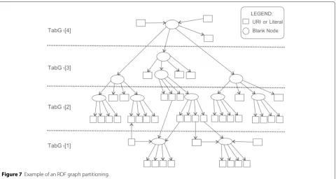
roots, leaves, intermediates, or no interconnections. We use the operator ‘[ ]’ to index the partitions ofTabGk, whereTabGk[i] denotes partitioniofTabGk.
Bnodes without links to other bnodes are placed in TabGk[ 1]. In the case of directly connected bnodes, the division thereof occurs according to a hierarchical model as shown in Figure 7.TabGk[ 4] contains bnodes that are roots in this model; TabGk[ 2] stores leaf bnodes; and TabGk[ 3] contains bnodes that belong to intermediate layers of this hierarchy, connected to other bnodes by both incoming and outbound links. For simplicity, in Figure 7, we omit the labels of the elements. Moreover, despite the presence of URIs and literals in the figure, the partitioning covers only blank nodes.
Each partition ofTabGk is further partitioned in a sec-ond level and indexed by the number of bnode links. This allows us to find bnodes with the same number of predi-cates quickly, whereTabGk[i] [j] returns a reference to the set of bnodes from partitioniofTabGk, withjconnections with neighboring nodes.
The ApproxMap algorithm also makes use of four arrays, with size equal to|Bk|, for each graphGk:aliask, approxInfk,approxSupk, andMk. Considering that bi ∈ Bk, aliask[i] stores the bnode currently mapped to bi; approxInfk[i] andapproxSupk[i] refer, respectively, to the values of the lower and upper approximations, calculated for bi and aliask[i]. Similarly, Mk[i] stores the bnode definitely mapped tobi.
Before describing the ApproxMap method, we need to explain the process of finding bnode pairs with the greatest approximation during the mapping. In the next section, we discuss this process, which uses the data structures mentioned above.
Mapping bnode pairs
We implemented the mapping of bnodes in two RDF graphs in two phases. In the first phase, as shown in the pseudocode in Figure 8, we look for pairs of unmapped bnodes with the closest approximation. The FindApprox-imationsalgorithm takes as parameters, indexesmandn referring, respectively, to the desired partitions ofTabG1
andTabG2, with 1 ≤ m,n ≤ 4, and parameterapprox,
where 0.0 < approx < 1.0, which denotes the lower boundary of the current desired approximation.
The algorithm looks for pairs with a value for the qual-ity of lower approximation γAinf(Xi,Xj) greater than or
equal to the desired value indicated by approx; values below this limit are discarded. Variablebmstores the cur-rent bnode with the closest approximation to bi, while apim and apsm store, respectively, their lower and upper approximations, calculated by metrics γAinf(Xi,Xj) and γAsup(Xi,Xj).
Considering subgraph Gi ⊆ Gk, as defined in
Equation 16,|Gi|is the cardinality ofGi, i.e., the number of triples or connections ofbi. In addition,iis the set of possiblepvalues for triples in the form(s,p,bi)∈Gi, and iis the set ofpvalues for triples(bi,p,o)∈Gi.
In lines 5 and 6 of the algorithm, we use the values of variableslinfandlsup to reduce the comparison space
using the top-down approximation approach discussed in the ‘Heuristic strategies’ subsection. We can only find an approximation greater than or equal to approx in the interval [linf,lsup], considering our second partitioning
level. In line 10, a further filtering takes place, whereby
only bnodes with at least one predicate in common are compared.
After obtaining the lower approximation betweenbiand the candidate bj, in line 16, we check whether this new approximation is greater than that previously found. If so, the respective bnodes are marked as candidates for mapping, and any previous pairs are discarded. However, if the new value for γAinf(Xi,Xj) is equal to that previ-ously found, we compare the new value ofγAsup(Xi,Xj), as shown in line 22. If this value is greater than the current value, the respective bnodes are also marked as candidates for mapping.
After the first phase, we have pairs of candidates
with the greatest approximation for mapping,
which is finalized in the second phase. Procedure MapApproximations(m,approx), with 1≤m≤4, is used to carry out the mapping. Bnodes in TabG1[m] with an
approximation greater than or equal to parameter approx are permanently mapped.
Procedures FindApproximations and
MapApproxima-tions are executed to map similar bnodes. However, we can refine these procedures to filter unmapped bnodes, when looking for equivalent pairs to reduce the search space. Thus, we designed procedureMapEquivalents(m) to map equivalent bnodes in TabG1[m] andTabG2[m],
where 1≤m≤4. This procedure compares only bnodes with exactly the same incoming and outbound predicates. Thus, we permanently map only those bnode pairs with approximations equal to 1.0.
We also developed a procedure to map the remain-ing bnodes, after termination of the iterations for the adopted top-down approximation strategy. Procedure MapByOrder()compares bnodes in the same way as Find-Approximations. However, the mapping is carried out directly between pairs with the greatest approximation according to the order defined by the partitioning of TabG1, thereby ignoring the possibility of a closer
rela-tionship with another bnode pair.
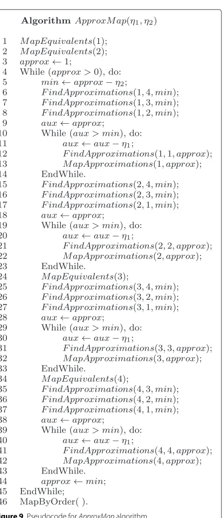
Proposed method
Finally, we present method ApproxMap illustrated in Figure 9, which aims to map the bnodes of two graphs G1andG2, considering a decreasing approximation in the
interval(0.0, 1.0). The mapping occurs between pairs in the same hierarchical levelTabG1[m] andTabG2[m]
con-sidering a fixed step defined by parameter η1. To map
bnodes of TabG1[m] and TabG2[n], with m = n, we
adopted the step defined byη2, where 0 < η1 < η2< 1.
Variable min stores the current desired value (or the lower boundary) for the approximation between bnodes.
TheApproxMapstarts by mapping equivalent bnodes in TabGk[ 1] andTabGk[ 2], as shown in lines 1 and 2. Dur-ing the mappDur-ing ofTabGk[ 2], we consider relaxing the neighboring bnodes for inbound links. This mapping is
Figure 9Pseudocode forApproxMapalgorithm.
performed only once, because these bnodes are leaves in the hierarchy and do not depend on previous mappings of other bnodes.
algorithm aims to mapTabG1[ 1] (lines 6 to 14),TabG1[ 2]
(lines 15 to 23),TabG1[ 3] (lines 24 to 33), andTabG1[ 4]
(lines 34 to 43) in order.
Thus, for each iteration of the outer loop, the value of min is decremented according to step η2, as expressed
in line 5. This value defines the minimum approximation required to map the bnodes in each partition ofTabG1to
the other different partitions inTabG2. In the case of the
same partitions, the mapping occurs in the inner loops, taking into account stepη1, so that the current
approxima-tion is decremented in each iteraapproxima-tion (lines 11, 20, 30, and 40), until it reaches the limit set inmin. Just prior to termi-nation of the algorithm, in line 46, the remaining bnodes are mapped after 1/η1iterations.
We compared the bnodes ofTabG1[m] 1/η1times with
the ones in TabG2[m], and a minor number of 1/η2
times with those inTabG2[n], wherem = n. Therefore,
during the search for bnode pairs with greater approxima-tions, the outer loop provides the mapping of bnodes that change partitions between versions, while the inner loop provides the mapping of bnodes that remain in the same hierarchical partition for all versions.
Method analysis
The proposed method models bnodes as approximate sets, based on their classification as equivalent, similar, or distinct predicates in terms of their connections with other nodes. This organization by approximation classes allows the definition of metrics to measure the approxi-mation between bnodes.
Considering the introductory example in Figure 1, algo-rithmsAlgHungandAlgSignobtain a mapping resulting in a delta with size 4. Tzitzikas et al. focused on the mapping between pairs(_:1, _:6)and(_:2, _:7)because they consid-ered connected bnodes to be the same, where disth(1, 6)= 0 and disth(1, 7)=1. We emphasize the adoption of both bottom-up and different neighbor strategies in Approx-Mapwhile mapping directly connected bnodes. The first iteration ofApproxMapresults in the mapping of bnode pairs(_:3, _:8),(_:4, _:10), and(_:5, _:9), which have an approximation equal to 1.0. From this initial mapping, our method can map pairs(_:1, _:7) and(_:2, _:6), because γAinf(X1,X6)=0.50,γAinf(X1,X7)=0.67,γAinf(X2,X6)=
0.67, andγAinf(X2,X7) = 0.34. The mapping obtained by
our method results in a smaller delta size of two triples.
On the other hand, during the ApproxMap method
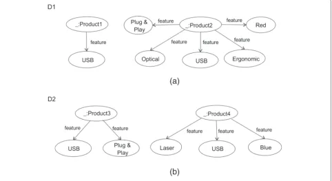
design, we assume that reducing the delta for individual bnode pairs also results in a reduction in the global delta size. However, this assumption does not produce the opti-mal delta in some situations, as illustrated in Figure 10. In this example, we assume that sets X1, X2, X3, and
X4 represent, respectively, bnodes ‘_:Product1’, ‘
_:Prod-uct2’, ‘_:Product3’, and ‘_:Product4’. Thus, we obtain the following approximation measurement: γAinf(X1,X3) =
0.50; γAinf(X1,X4) = 0.33; γAinf(X2,X3) = 0.40; and
γAinf(X2,X4)=0.14.
First, ApproxMap maps bnodes ‘_:Product1’ and
‘_:Product3’, corresponding to the pair with the clos-est approximation. The closclos-est approximations of both ‘_:Product1’ and ‘_:Product2’ are to bnode ‘_:Product3’.
However, this mapping represents the lowest cost of transforming some bnode in the first version into ‘_:Product3’. We can change ‘_:Product1’ to ‘_:Product3’ by including only a single triple. However, we would need to include an additional three triples to transform ‘_:Product2’ into ‘_:Product3’.
Therefore,ApproxMapalso maps the remaining bnodes ‘_:Product2’ and ‘_:Product4’, resulting in a global delta containing seven triples. However, if we had initially mapped ‘_:Product1’ to ‘_:Product4’, the resulting delta would have size 5, as is the case using theHungarian algo-rithm. This occurs because our hypothesis considers only a reduction in delta between individual pairs and not an assessment of the impact of this reduction in terms of the global delta size. Owing to the mapping of remain-ing bnodes, considerremain-ing only unmapped bnodes pairs, the ApproxMapdoes not test all mapping possibilities, which can result in obtaining a local optimum.
Moreover, in ApproxMap, the mapping occurs in the order defined by the adopted partitioning. We also used some ordered structures during algorithm implementa-tion, optimizing the comparisons between bnodes. The additional cost of insertion is already known for these structures, although this is beyond the scope of this arti-cle. This adopted order can affect the delta size, mainly, considering procedureMapByOrder. As before, this may occur because our method does not test all mapping possibilities.
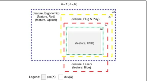
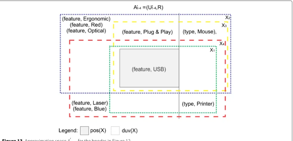
We emphasize that great diversity among the bnode predicates in the same version is beneficial for method ApproxMap. For a better analysis, let us consider the approximation space A1−4, illustrated in Figure 11, and
which we constructed from the union of all sets represent-ing bnodes in the two versions in Figure 10. For simplicity, we omit the negative regions of the bnodes in Figure 11.
According to Figure 11, there are few differences between sets of the same version. In particular, X1 is a
subset of all other sets, hindering the choice of its best mapping option. The inclusion of different values can con-tribute to a better choice of bnode pairs, as illustrated in Figure 12.
Figure 13 illustrates the approximation spaceA1−4, con-sidering all bnodes in the datasets in Figure 12. Now, the bnodes within the same version have greater diver-sity, allowing a better approximation measure between bnodes if we consider the different versions. In this case, the new values of predicate ‘type’ leads to a better choice of the candidates, where we haveγAinf(X1,X3) =
0.25; γAinf(X1,X4) = 0.5; γAinf(X2,X3) = 0.5; and
γAinf(X2,X4) = 0.11. Thus, the new delta obtained from
ApproxMapcontains five triples.
In particular, it may be difficult for ApproxMap to choose the best mapping option if there are multiple candidates representing approximately equal sets in an approximation space, i.e., sets with the same lower and upper approximations [7], as exemplified in Figure 14a.
Figure 12 Sample datasets with greater diversity between bnodes(a,b).
The adopted metrics may be insufficient to distinguish these sets.
Furthermore, in cases involving completely different datasets, ApproxMap compares all bnodes in the two datasets during the mapping, resulting in the maximum
delta equal to the sum of the triples in the two datasets. We included some optimizations inApproxMap, reduc-ing the cost of comparreduc-ing distinct pairs, by first checkreduc-ing for the presence of common predicates. The worst-case execution corresponds to a particular case of distinct
Figure 14Approximately equal sets and a dispersed set(a,b).
datasets, where all bnodes have the same predicates. In this case, we obtain dispersed approximate sets represent-ing the bnodes, i.e., sets with an empty lower approxima-tion (γAinf(Xi,Xj)=0) and an upper approximation equal to the set universe (γAsup(Xi,Xj) = |U|) [7], as shown in Figure 14b.
We use stepη1to control the number of comparisons
between bnodes, where the total number is given by 1/η1×O(n2). Thus, whenη1is considerably smaller than
1/n, wherengives the smallest number of bnodes in the datasets, in the worst case, the time complexity of the algorithm is O(n2). Conversely, the best case execution
ofApproMapoccurs with equivalent datasets containing bnodes with varying numbers of connections and without any directly connected bnodes. In this case, we need to compare each bnode with exactly one bnode in the other version. Thus, the complexity of the best case is (n).
Finally, we intend to applyApproxMapto configuration management of software engineering projects, specifically to version control of RDF datasets. These projects are characterized by the manipulation of data, information, and knowledge in various types and formats, manually constructed based on the modularity principle, where complex elements are divided into smaller parts. There-fore, we expect great diversity between bnodes in the same version, justifying the application of ApproxMapin this context.
Because the datasets involved are usually constructed using an incremental development approach, we expect satisfactory performance of ApproxMap on similar ver-sions, containing several approximately equivalent bnode pairs, as generally occurs in successive versions of soft-ware engineering artifacts. A recommended configuration management practice is to perform version control con-sidering the low percentage of changes between versions. If this does not occur, larger deltas prevent the recovery of intermediate states between successive versions.
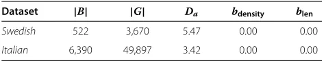
Table 1 Information about real datasets
Dataset |B| |G| Da bdensity blen
Swedish 522 3,670 5.47 0.00 0.00
Italian 6,390 49,897 3.42 0.00 0.00
As future work, we propose a meticulous analysis of the impact of the adopted metrics and strategies on the map-ping. We also intend verifying the applicability of other RST metrics that could provide better approximation measures between bnodes. As a further future work, we propose improving the performance of the algorithm, tak-ing into account execution of some operations in parallel, such as comparison of approximate sets.
Results and discussion
In analyzing the performance of the ApproxMap algo-rithm, we considered both the delta size calculated from mapping pairs of RDF datasets and the time spent on this task. This allowed comparison of the results and values obtained for theAlgHungandAlgSignalgorithms, presented by Tzitzikas et al. [6]. All experiments discussed in this section were executed on an Intel Core i7-3537U, 2.0 GHz processor, with 8 GB RAM and running Ubuntu 13.10. To correct any formatting or encoding issues, preprocessing was carried out on certain pairs of datasets.
Three metrics defined by Tzitzikas et al. [6] were used in the analysis of the experiments:bdensity, blen, andDa. Let N andBdenote, respectively, the sets of nodes and blank nodes of graphG, whereB⊆N. Further, let conn(b) denote the set of nodes inGdirectly attached tob ∈ N. Then, we havebdensity=avgb∈B(|conn(b)∩B|/|conn(b)|);
blen refers to the average maximum path length, with
Table 2 Results of the algorithms applied to real datasets
Dataset Swedish Italian
Delta(triples)
ApproxMap1/10% 297 6
ApproxMap5/12% 297 6
ApproxMap5/25% 297 6
AlgHung 297 6
AlgSign 423 6
Time(ms)
ApproxMap1/10% 113 170
ApproxMap5/12% 36 158
ApproxMap5/25% 34 153
AlgHung 4,789 456,173
Table 3 Crawled datasets using the load-balancing strategy
Instance number |B| |G| Da bdensity blen
1 19 1,048 9.00 0.01 0.11
2 83 11,555 7.31 0.00 0.00
3 361 28,208 5.93 0.00 0.00
4 362 28,219 5.96 0.00 0.00
5 893 15,337 4.40 0.00 0.02
vertexes consisting only of bnodes; andDacorresponds to the average number of bnode triples.
Except for the last experiment, we tested the Approx-Map algorithm with three different sets of parameters: η1 = 0.01 andη2 = 0.1;η1 = 0.05 andη2 = 0.125; and
η1 = 0.05 andη2 = 0.25 where these tests are denoted,
respectively, asApproxMap 1/10%, ApproxMap 5/12%, andApproxMap5/25%. We chose these steps empirically, considering the desired number of iterations. As future work, we propose further analysis of the choice of step values and calibration ofApproxMap.
We used theApproxMap 5/12% tests as the baseline for comparison when evaluating the impact of changes in η1 and η2 on the results. The ApproxMap 5/12%
test includes 20 iterations (1/η1) of the inner loop of
the method, comparing each bnode with those in the same hierarchical partition in the second version. In addi-tion, there are eight iterations (1/η2) of the outer loop,
comparing the bnodes with those in the remaining par-titions. The ApproxMap 5/25% test was used to verify the impact of an increase in η2, reducing the
compar-isons between distinct partitions for 4 iterations. Finally, we used theApproxMap1/10% tests to analyze the impact of a reduction inη1, increasing the comparisons between
the same partitions for 100 iterations. In these tests, we
also adjustedη2to better fitη1, resulting in ten iterations
of the outer loop.
We organized the experiments in three groups based on the type of dataset used in each: real, extracted from the Web (i.e., crawled), or synthetic datasets, as discussed in the following sections. The standard units for delta size and mapping time are, respectively, triples and mil-liseconds. We used a logarithmic scale for charts showing mapping times of the algorithms, thereby providing better visualization and comparison of the results.
Real datasets
In the first group of experiments, we used the same real datasets tested by Tzitzikas et al. [6]. Table 1 describes the main features of these datasets, where columns|B|and|G| denote, respectively, the average numbers of bnodes and triples in the version pairs. Measurements for the dataset Italianare the same for both files. In theSwedishdataset, the coefficient of variation (cv) is equal to 2.42%, 2.98%, and 0.19%, for|G|,|B|, andDa, respectively.
Table 2 gives the results obtained by the algorithms in the first experiment, considering the time to map blank nodes and the delta size calculated from this mapping. In terms of the delta, we obtained the same values for both datasets in all algorithm tests, with the exception of AlgSign. With respect to the execution time, considering the ratio between the time of the algorithmsAlgHung and ApproxMap 5/25%, we obtained 141 and 2,982, respec-tively, for theSwedishandItaliandatasets. Thus,AlgHung required considerable additional time, particularly for datasetItalian.
Crawled datasets
Owing to the difficulty in finding appropriate real ver-sioned datasets for the experiments, in the second group of experiments, we used an RDF crawler,LDSpider[21],
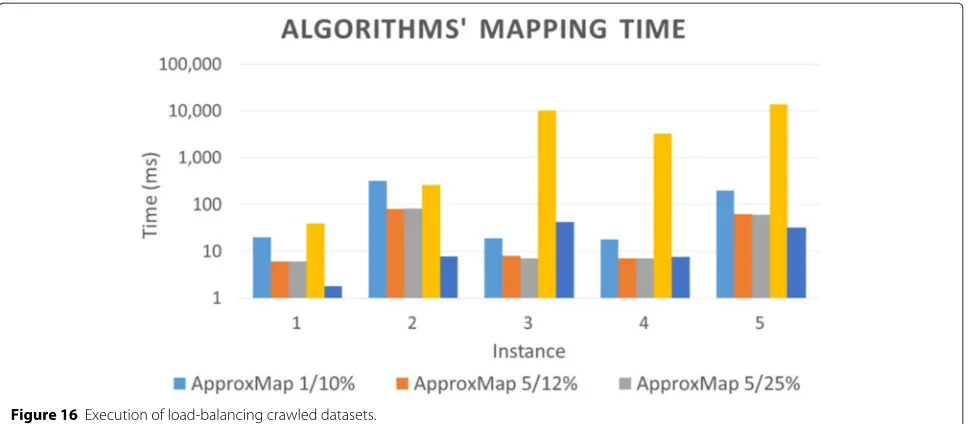
Figure 16Execution of load-balancing crawled datasets.
to construct pairs of RDF dataset versions. We extracted some versions from randomly chosen links to common datasets in the linked open data (LOD) cloud [22], such as Dbpedia and DBPL, as well as FOAF Profiles.
We used LDSpider because of its dual crawling strate-gies [21]: breadth-first and load-balancing. Thus, we exe-cuted two experiments based on these strategies, where the maximum number of URIs was limited to generate reasonably sized files for the tests, considering the com-putational costs of the algorithms. In the first experiment usingLDSpider, we adopted the load-balancing strategy, with the aim of obtaining pairs of files with approximately the same size. Table 3 gives information about the crawled datasets used. The first column denotes the instance num-ber. All values in Table 3 were identical for both produced versions, with the exception of metric|G| in the second instance, wherecv=0.73%.
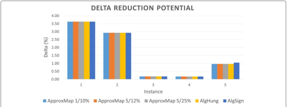
Figures 15 and 16 illustrate the results for the datasets described in Table 3. To further analyze the delta reduc-tion potential of the algorithms, the deltas are pre-sented as a percentage of the average number of triples, i.e., (G1,G2)/|G|. As seen in Figure 15, all algorithms
achieved the same delta reduction on all datasets, except
forAlgSign, which showed an increase of 0.08 in the delta reduction potential, in the last instance, compared with the potential of the other algorithms.
For bnode mapping, algorithm AlgHung was the slow-est. Considering the differences between the mapping times of the algorithms presented in Figure 16, compared with ApproxMap 5/25%,AlgHung showed an increase in mapping time between 0.50 and 3.16, on the adopted loga-rithmic scale.ApproxMap5/25% was faster thanAlgSignin two instances, with the maximum time increase forAlgSign equal to 0.78.AlgSignwas faster in the remaining instances, with an increase in time forApproxMap5/25% less than 1.03. Finally, considering the differences between stepsη1
andη2, compared withApproxMap5/12%, the mapping
time for ApproxMap 1/10% increased by between 0.38 and 0.60, while ApproxMap 5/25% showed a maximum reduction in mapping time of 0.06.
In the second experiment usingLDSpider, we extracted the first version using the breadth-first strategy and the second using the load-balancing strategy. Once again, we aimed to create files with approximately the same size but with major differences due to the change in strategy. Table 4 shows features of the instances considered in this
Table 4 Crawled datasets with breadth-first/load-balancing strategy
Instance number |B| |G| Da bdensity blen
File 1 File 2 File 1 File 2 File 1 File 2 File 1 File 2 File 1 File 2
1 169 19 4,355 1,048 5.73 9.00 0.21 0.01 16.26 0.11
2 190 83 11,892 11,470 5.82 7.31 0.07 0.00 1.67 0.00
3 1,246 893 24,364 15,337 5.13 4.40 0.10 0.00 10.88 0.02
4 1,963 361 27,650 28,208 6.75 5.93 0.00 0.00 0.00 0.00
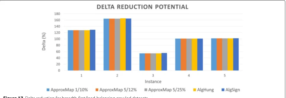
Figure 17 Delta reduction for breadth-first/load-balancing crawled datasets.
experiment. Detailed information is given in this table, because there are considerable differences between some versions.
Figure 17 shows the delta reduction potential of the algorithms in these tests.AlgHung showed an increase in its delta reduction percentage of 1.26, while the increase in potential ofAlgSignwas less than 1.42, when compared with all tests usingApproxMap.
Figure 18 compares the mapping times on a loga-rithmic scale. AlgHung once again performed the worst. Compared withApproxMap 5/25%, the mapping times of AlgHung increased by between 0.11 and 1.92. Com-pared with AlgSign, the increase in mapping times of ApproxMap5/25% varied between 0.46 and 1.59. Besides, we also verified a time increase for theApproxMaptests; the mapping time of ApproxMap 1/10% increased by between 0.42 and 0.60, while that ofApproxMap 5/25% decreased by 0.12 , compared withApproxMap5/12%.
Synthetic datasets
In this final group of experiments, to evaluate the algo-rithms in the mapping of datasets with some specific features, e.g., directly connected bnodes or equivalent datasets, we generated pairs of synthetic datasets for use in the tests.
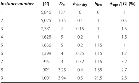
Datasets from adapted Univ-Bench artificial generator Initially, we considered the datasets used by Tzitzikas et al. [6], the generator of which was based on the Univ-Bench artificial (UBA) data generator [23]. Table 5 lists the features of the dataset pairs tested in this experiment, where all datasets have 240 bnodes. In this table, column opt/|G| displays the ratio between the optimal values,
represented byopt(G1,G2), and|G|. For the average
val-ues shown in this table, we havecv = 16.17% and cv = 1.3% toblen, respectively, for instances 4 and 9, andcv<
0.22% in the other cases.
Table 5 Synthetic datasets generated by Tzitzikas et al. [6]
Instance number |G| Da bdensity blen opt/|G|(%)
1 5,846 13.4 0 0 1
2 5,025 10.5 0.1 1 0.5
3 2,381 7 0.15 1 1.5
4 1,628 5 0.2 1 1.5
5 1,636 5 0.2 1.15 1
6 1,399 4 0.25 1.15 1.7
7 919 3 0.32 1.15 3.2
8 909 3.25 0.4 1.35 2.7
9 1,001 3.94 0.5 21.5 2.5
Figure 19 shows the delta sizes obtained for the nine version pairs. ApproxMap and AlgHung found the opti-mal delta in five instances.AlgHung found a smaller delta than ApproxMap 5/25% in instances 4 and 7, with the maximum decrease in delta equal to 0.65. More-over, in the latter instance, AlgHung was only surpassed by ApproxMap 5/25%. We confirmed the smallest delta reduction potential in instance 8, where ApproxMap, AlgHung, andAlgSign showed increases of 5.34, 7.98, and 8.86, respectively, when compared with the optimal reduc-tion potential.
Figure 20 shows the results for the same nine pairs but considering the second version in reverse order. Contrary to the results of the algorithms proposed by Tzitzikas et al. [6], the bnode order did not affect the results of Approx-Map. For the final four instances, compared with the optimal reduction potential,AlgHung showed an increase varying from 6.72 to 19.64. Similarly, for these instances, the increase in the reduction potential of AlgSign varied from 8.86 to 20.75, compared with the optimal values.
Figure 21 shows the results for the mapping times of the algorithms on a logarithmic scale. AlgHung
achieved the worst performance, with increased map-ping time varying between 1.53 and 2.45, compared with ApproxMap 5/25%. In the final three instances, AlgSign achieved better performance than ApproxMap 5/25%, with decreased mapping time of between 0.12 and 0.65. ApproxMap5/25% performed better in the first instance, executing faster than AlgSign with a decrease in time of 0.98. Finally, compared with ApproxMap 5/12%, the
mapping time of ApproxMap 1/10% showed a
maxi-mum increase of 0.52, while that ofApproxMap 5/25% decreased by 0.16.
Datasets with directly connected bnodes
In the final three instances of the nine pairs of synthetic datasets used above, all algorithms obtained higher deltas than the optimal values, when applied to datasets with a marked increase in the number of directly connected bnodes. To assess the influence ofbdensityon delta size, we
conducted a new experiment with identical versions of the datasets. All algorithms found an empty delta for the orig-inal order of the datasets. However, considering a reverse order in the second version, Figure 22 shows the results in terms of the deviation from the optimal delta, i.e., dx= (G1,G2)−opt(G1,G2)
opt(G1,G2)+1 , whereoptdenotes the optimal
value. With an increase in bdensity, the reverse ordering
once again influenced the results of AlgHung andAlgSign. These algorithms achieved the same increase indxin the final three instances, whereas ApproxMap produced an empty delta.
To analyze the performance of the algorithms, consid-ering datasets with a higher number of directly connected bnodes, we developed an RDF dataset generator, based on that included in the Berlin SPARQL Benchmark (BSBM) [24]. We used this generator to produce pairs of file ver-sions with an averagebdensityof 0.34%, andcv=7.25%. We
discuss the experiments using this generator in the next section.