RESEARCH
How Amdahl’s Law limits the performance
of large artificial neural networks
why the functionality of full-scale brain simulation on processor-based simulators is
limited
János Végh
*Abstract
With both knowing more and more details about how neurons and complex neural networks work and having serious demand for making performable huge artificial networks, more and more efforts are devoted to build both hardware and/or software simulators and supercomputers targeting artificial intelligence applications, demanding an exponentially increasing amount of computing capacity. However, the inherently parallel operation of the neural networks is mostly simulated deploying inherently sequential (or in the best case: sequential–parallel) computing ele-ments. The paper shows that neural network simulators, (both software and hardware ones), akin to all other sequen-tial–parallel computing systems, have computing performance limitation due to deploying clock-driven electronic circuits, the 70-year old computing paradigm and Amdahl’s Law about parallelized computing systems. The findings explain the limitations/saturation experienced in former studies.
Keywords: Amdahl’s Law, Neural networks, Performance limitation, Clock-driven electronic circuit, Supercomputing, Parallelization
© The Author(s) 2019. This article is distributed under the terms of the Creative Commons Attribution 4.0 International License (http://creat iveco mmons .org/licen ses/by/4.0/), which permits unrestricted use, distribution, and reproduction in any medium, provided you give appropriate credit to the original author(s) and the source, provide a link to the Creative Commons license, and indicate if changes were made.
1 Introduction
Although von Neumann in his classic publication [1, 2] targeted creating computing organs, developers had to consider the that-time technological possibilities and the urgent need to automate numeric calculations. In this way, the primary goal was to compute and all efforts (at that time and the next seven decades) were devoted to develop the device computer. The sound success of that automated computing and the growing scientific, indus-trial, military, etc. needs targeted to increase the single-processor performance, although more than five decades ago it was already recognized [3] that when utilizing that computing principle one faces serious performance limi-tations. The today’s goal to simulate operation of even a relatively small-scale (compared to human brain) neu-ral network in real-time faces serious difficulties and leads to serious performance issues [4]. In the light of
that biological neurons work in the millisecond range, the silicon neurons could work in the nanosecond range and that both software-only neural network simulator programs running on supercomputers built from gen-eral-purpose processors and special-purpose hardware brain-simulator utilize million(s) of high-performance processors produce such a low performance, the question raises: where do we loose several orders of magnitude of computing performance?
One obvious candidate for loosing performance is the general-purpose processor itself [5]: its performance is awfully low compared to implementation in Applica-tion Specific Integrated Circuits. However, it cannot be responsible alone for the full loss. The development of single-processor performance has stalled [6] and only marginal development of single-processor performance can be expected. The computing needs renewing [7, 8] because of many reasons. One of them is that the many forms of increasing the performance through various kinds of parallelization [9] is a short dead-end street: the computing efficiency exponentially decreases as the
Open Access
number of processors increases [10], the today’s super-computers are stretched to their limits [11] in the case of large-scale systems. A slowdown or stalling of the growth of their performance is expected according to the general experiences [12] and is really experienced among others in the field of supercomputing [13]. However, similarly to most of the basic limitations of computing, even the limi-tations are limited [14].
The goal of the paper is to show that akin to super-computers the computing performance of the proces-sor-based brain simulators is also limited. As discussed below, utilizing (mainly: thinking in) clocked electronic circuits, the 70-year-old single-processor approach and Amdahl’s Law together result in that only marginal devel-opments in the performance of neuromorphic simula-tions can be expected. The question only is how far brain simulation is from its limitations? And of course, whether those limitations are limited, too?
The paper first interprets Amdahl’s Law for any kind of parallelized activity in Sect. 2 and shows in Sect. 3 that utilizing clock signals in the electronic circuits leads to an inherent limitation of performance. Section 4 shows how in supercomputing this inherent limitation bounds the achievable computing performance. Although brain simulation seems to be unrelated to the sequential/paral-lel computing world, in Sect. 5 it is shown that the tech-nical implementation introduces a hidden clock signal into neural computing. This section also reveals the ori-gins of the saturation effects experienced in former stud-ies. Finally, in Sect. 6, some ideas are proposed for using some alternative approach to get closer to full-power brain simulations.
2 Amdahl’s Law of parallelization 2.1 Amdahl’s idea
Amdahl’s Law is one of the few, fundamental laws of com-puting [15], although sometimes it is partly or completely misinterpreted or abused [15–17]. A general misconcep-tion (introduced by successors of Amdahl) is to assume that Amdahl’s law is valid for software only. Actually,
Amdahl’s law is valid for any partly parallelizable activ-ity (including computer unrelated ones) and the non-par-allelizable fragment shall be given as the ratio of the time spent with non-parallelizable activity to the total time. Notice that Amdahl speaks about partly parallelizable activities in simple parallelized systems, unlike complex sequential–parallel systems with variable degree of paral-lelism [18] or the brain operation. That is, Amdahl’s law can be directly applied only to such simple systems, but the idea itself can be utilized to study even the mentioned complex systems.
2.2 Deriving the effective parallelization
Successors of Amdahl expressed Amdahl’s law with the formula
where k is the number of parallelized activities, α is the
ratio of the parallelizable part within the total activity, S
is the measurable speedup. The assumption can be visu-alized that (in a conventional computing system assum-ing many processors) in α fraction of the running time
the processors are executing parallelized code, in ( 1−α )
fraction they are waiting (all but one), or making non-payload activity. That is α describes how much, in
aver-age, processors are utilized, or how effective (at the level of the computing system) the parallelization is.
For a system under test, where α is not a priory known,
one can derive from the measurable speedup S an effec-tive parallelization factor [19] as
Obviously, this is not more than α expressed in terms
of S and k from Eq. (1). For the classical case, α =αeff ;
which simply means that in the ideal case the actually measurable effective parallelization achieves the theoreti-cally possible one. In other words, α describes a system
the architecture of which is completely known, while αeff
characterizes the performance, which describes both the complex architecture and the actual conditions. It was also demonstrated [19] that αeff can be successfully
uti-lized to describe paralleuti-lized behavior from software (SW) load balancing through measuring efficacy of the on-chip communication inside a hardware (HW) unit to characterizing performance of clouds.
The value αeff can also be used to refer back to
Amdahl’s classical assumption even in the realistic case when the parallelized chunks have different lengths and the overhead to organize parallelization is not negligible. The speedup S can be measured and αeff can be utilized
to characterize the measurement setup and conditions, how much from the theoretically possible maximum par-allelization is realized. Numerically ( 1−αeff ) equals with
the f value, established theoretically [20].
The distinguished constituent in Amdahl’s classic anal-ysis is the parallelizable fraction α , all the rest
(includ-ing wait time, non-payload activity, etc.) goes into the “sequential-only” fraction. When using several proces-sors, one of them makes the sequential calculation, the others are waiting (use the same amount of time). So, when calculating the speedup, one calculates
(1)
S−1=(1−α)+α/k
(2)
αeff =
k k−1
S−1
S
(3)
S= (1−α)+α (1−α)+α/k =
hence the efficiency is (see also Fig. 2).
This explains the behavior of diagram S
k in function of k experienced in practice: the more processors, the lower efficiency. At this point, one can notice that 1
E is a linear
function of number of processors, and its slope equals to (1−α) . Equation (4) also underlines the importance of the single-processor performance: the lower is the num-ber of the processors used in the parallel system having the expected performance, the higher can be the efficacy of the system.
Notice also, that through using Eq. (4), the efficiency S k (which is given for supercomputers as RMax
RPeak ) can be equally good for describing the efficiency of paralleliza-tion of a setup, provided that the number of processors is also known. From Eq. (4)
If the parallelization is well-organized (load balanced, small overhead, right number of processors), αeff is close
to unity, so tendencies can be better displayed through using (1−αeff) in the diagrams.
The importance of this practical term αeff is underlined
by that it can be interpreted and utilized in many differ-ent areas [19] and the achievable speedup (the maximum achievable performance gain when using infinitely large number of processors) can easily be derived from Eq. (1) as
Provided that the value of αeff does not depend on the
number of the processors, for a homogenous system the total payload performance is
i.e., the total payload performance can be increased by increasing the performance gain or increasing the single-processor performance, or both. Notice, however, that increasing the single-processor performance through accelerators also has its drawbacks and limitations [21], and that the performance gain and the single-processor performance are players of the same rank in defining the payload performance.
Notice the special role of the non-parallelizable activi-ties: independently of their origin, they are summed up as ‘sequential-only’ contribution and degrade considerably the payload performance. In systems comprising paral-lelized sequential processes actions like communication
(4)
E = S
k =
1
k(1−α)+α
(5)
αE,k = Ek−1
E(k−1)
(6)
G= 1
(1−αeff)
(7)
Ptotal payload=G·Psingle processor
(including also MPI), synchronization, accessing shared resources, etc. [22–25] all contribute to the sequential-only part. Their effect becomes more and more drastic as the number of the processors increases. One must take care, however, how the communication is implemented. A nice example is shown in [26], how direct core to core (in other words: direct thread to thread) communication can enhance parallelism in large-scale systems.
3 The inherent limit of parallelization
In the systems implemented in single-processor approach (SPA) [3] as parallelized sequential systems, the life begins in one such sequential subsystem. For example, in large parallelized applications running on general-pur-pose supercomputers, initially and finally only one thread exists, i.e., the minimal absolutely necessary non-parallel-izable activity is to fork the other threads and join them again. With the present technology, no such actions can be shorter than one processor clock period.1 That is, the absolute minimum value of the non-parallelizable frac-tion will be given as the ratio of the time of the two clock periods to the total execution time. The latter time is a free parameter in describing the efficiency, i.e., value of the effective parallelization αeff also depends on the total
benchmarking time (and so does the achievable paralleli-zation gain, too).
This dependence is of course well known for super-computer scientists: for measuring the efficiency with better accuracy (and also for producing better αeff
val-ues) hours of execution times are used in practice. For example, in the case of benchmarking the supercomputer
Taihulight [27] 13,298 s benchmark runtime was used; on
the 1.45 GHz processors it means 2∗1013 clock periods. This means that (at such benchmarking time) the inher-ent limit of (1−αeff) is 10−13 (or equivalently the achiev-able performance gain is 1013 ). If the fork/join is executed by the operating system (OS) as usual, because of the needed context switchings 2∗104 [28] clock cycles are
needed rather than the 2 clock cycles considered in the idealistic case, i.e., the derived values are correspondingly by 4 orders of magnitude different; that is the performance gain cannot be above109 . When making only 10 s long
measurements, the smaller denominator results in 103 times worse (1−αeff) and performance gain values. In the following for simplicity 1.00 GHz processors (i.e., 1 ns clock cycle time) will be assumed.
There are other similar limitations in consequence of the physical implementation. The supercomputers,
for example, are also distributed systems. In a stadium-sized supercomputer, the distance between processors (cable length) about 100 m can be assumed. The net sig-nal round trip time is ca. 10−6 s, or 103 clock periods, i.e., in the case of a finite-sized supercomputer the per-formance gain cannot be above 1010 (or 106 if context switching also needed). The presently available network interfaces have 100...200 ns latency times, and sending a message between processors takes time in the same order of magnitude. This also means that making better interconnection is not really a bottleneck in enhancing performance, at least when measured using the bench-mark High-Performance Linpack (HPL). This statement is underpinned also by statistical considerations [21].
Taking the (maybe optimistic) value 2∗103 clock peri-ods for the signal propagation time, the value of the effec-tive parallelization (1−αeff) will be at best in the range of 10−10 , only because of the physical size of the
supercom-puter. This also means that the expectations against the absolute performance of supercomputers are excessive: assuming a 100 Gflop/s processor, the achievable absolute
nominal performance (see Eq. (6)) is 1011*1010flop/s , i.e., 1000 EFlops. To implement this, around 109 processors
are required. One can assume that the value of (1−αeff) will be2 around of the value 10−7 . With those very opti-mistic assumptions (see Eq. 4), the payload performance for benchmark HPL will be less than 10 Eflops, and for the real-life applications of class of the benchmark High-Performance Conjugate Gradients (HPCG), it will be surely below 0.01 EFlops, i.e., lower than the payload per-formance of the present TOP1-3 supercomputers.
These predictions enable to assume that the presently achieved value of (1−αeff) persists also for roughly hun-dred times more cores. However, another major issue arises from the computing principle single-processor approach (SPA): only one computer at a time can be addressed by the first one. As a consequence, minimum as many clock cycles are to be used for organizing the parallel work as many addressing steps required. Basi-cally, this number equals to the number of cores in the supercomputer, i.e., the addressing in the TOP10 posi-tions typically needs clock cycles in the order of 5∗105 ...107 ; degrading the value of (1−αeff) into the range 10−6 ...2∗10−5 . Two tricks may be used to mitigate the
num-ber of the addressing steps: either the cores are organ-ized into clusters as many supercomputer builders do, or at the other end the processor itself can take over the responsibility of addressing its cores [29]. Depending on
the actual construction, the reducing factor of cluster-ing of those types can be in the range 102...5∗104 , i.e., the resulting value of (1−αeff) is expected to be around
10−7 . Notice that utilizing “cooperative computing” [29]
enhances further the value of (1−αeff) , but it means already utilizing a (slightly) different computing para-digm: the cores have a kind of direct connection and can communicate with the exclusion of the main memory.
An operating system must also be used, for protection and convenience. If one considers context switching with its consumed 2∗104 cycles [28], the absolute limit is cca.
5∗10−8 , on a zero-sized supercomputer. This value is
somewhat better than the limiting value derived above, but it is close to that value and surely represents a con-siderable contribution. This is why Taihulight runs the actual computations in kernel mode [29].
Because all of this, in the name of the company PEZY3, the last two letters are surely obsolete. Also, no Zetta-flops supercomputers will be delivered for science and military [30]. It looks like that in the feasibility studies, an analysis on whether this inherent performance bound exists is done neither in USA [31] nor in EU [32] nor in Japan [33] nor in China [13].
As discussed above, some limitations follow immedi-ately from the physical implementation and the comput-ing paradigm; it depends on the actual conditions, which of them will dominate. It is crucial to understand that the decreasing efficiency (see Eq. (4)) is coming from the computing paradigm itself rather than from some kind of engineering imperfectness. This inherent limitation cannot be mitigated without changing the computing/implemen-tation principle.
4 The inherent limits of supercomputing
The considerations on supercomputing result in a (by intention oversimplified) parametrized model that quali-tatively describes the behavior of the supercomputers during its 26 years of history, and the parameters can be estimated from the public, rigorously controlled, accurate database [34]. The model [10, 35] not only describes the performance of the presently existing supercomputers, but also predicts their future achievable performance.
Although not explicitly dealt with here, notice that the data exchange between the first thread and the other ones also contribute to the non-parallelizable fraction and typ-ically uses system calls, for details see [23–25]. Actually, we may have communicating serial processes, which does not improve the effective parallelism at all [22]. Essen-tially, this is why supercomputers have a “benchmark
2 With the present technology the best achievable value is ca. 10−6
, which was successfully enhanced by clustering to ca. 2∗10−7
for Summit and Sierra , and the special cooperating cores of Taihulight enabled to achieve 3∗10−8
.
efficiency” (measured by HPL) and a “practical efficiency” (measured by benchmark HPCG), the latter of which is 100...1000 times lower than the former one. For details see [10]. Recall that artificial neurons make intensive data exchange among each other, so they surely belong to the HPCG class of applications, although utilizing “far” and “near” memories can change their behavior drastically.
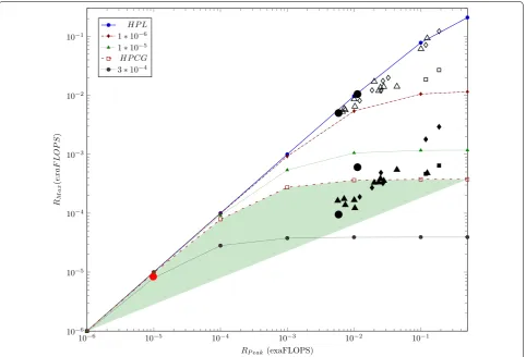
Figure 1 depicts how the payload performance of the benchmarks HPL and HPCG depend on the nominal performance of the general-purpose supercomputers. The diagram lines referring to different (1−αeff) val-ues are calculated from the model [10], the marks are measured for the different TOP15 supercomputers (as of Nov 2018). The empty marks refer to the HPL and the filled ones to the HPCG benchmarks. For more legends and explanations see [10]. Notice that the simulators of
artificial neural networks show up a behavior quite close to the HPCG class applications, see below.
5 The inherent limits of neural network simulation Of course, brain simulation as such has nothing to do with clock-driven sequential-parallel processing. How-ever, brain simulators (the SW ones and most of the HW ones) run on such computing systems (are built from such components) and inherit the limitations valid for those systems. As discussed above, Eq. (7) defines the achievable payload performance of a parallelized com-puting system, and also that the performance gain is lim-ited by the clock frequency.
The living “architectures” have no central clock sig-nal, so the simulations should not have one, too. Despite this, from technology reasons, all simulations utilize a
10−6 10−5 10−4 10−3 10−2 10−1
10−6 10−5 10−4 10−3 10−2 10−1
RP eak (exaFLOPS) RMa
x
(
exaF
LO
PS
)
HP L 1∗10−6 1∗10−5 HP CG 3∗10−4
“time grid”, commonly with 1 ms integration time. This grid time is used to put the free running neurons back to the biological time scale, i.e., they actually act as a clock signal: stimulating of the next calculation step can only start when this clock signal arrives. This is absolutely analogous with the goal of introducing clock signal for executing the machine instructions: the processor, even when it is idle, cannot begin the execution of the next machine instruction until the clock signal arrives. The artificial neural networks constructed in this way can be considered as consisting from nodes having rather com-plex internal operation (implementing exceptionally high computing performance) and concerted by the clock sig-nal which is technically required to enable performing the concerted integration.
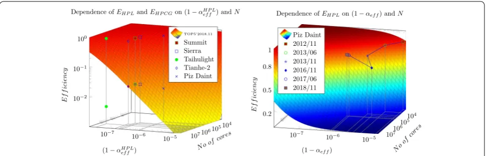
If the artificially introduced "biological clock cycle" is not considered (it introduces a new dimension), the payload efficiency depends on both the the efficiency of parallelization and the number of the processors in the system, as described by Eq. (4) and displayed in Fig. 2. Under the conditions of supercomputing, the expected high performance puts strong constraints both on the number of the processors and the efficiency of their par-allelization. As the figure displays, in order to get away from the strongly non-linear part of this 2-dimensional surface (i.e. to have a reasonable efficiency), the present (as of 2018 November) top 5 supercomputers must show up a good bargain between having large single-proces-sor performance and at the same time showing up good effective parallelism.
The figure shows also how the "benchmarking perfor-mance (HPL)" of the top 5 supercomputers are posi-tioned on the 2-dimensional surface, while the "real-life performance (HPCG)" values of the efficiency are of two orders of magnitude lower. It is crucial to see that increasing only the number of the cores has a reverse effect on the efficiency of the parallelization, and so leads to a decreasing payload performance, see the right side of Fig. 2. It is interesting to see that the unique HW solu-tion of Taihulight resulting in outstanding parallalizasolu-tion efficiency (especially at that high number of cores) works only when measured with HPL and it draws back when measuring with HPCG. Recall also, that the AI applica-tions are expected to have effciency about 1% (the typical efficiency of HPCG class), and introducing the "biologi-cal clock cycle" in brain simulation, decreases the effi-ciency further by 2-3 orders of magnitude.
5.1 The contribution from the “clock signal”
As discussed shortly in Sect. 3 and in more details in [35], the non-parallelizable fraction of the computing load sums up from different contributions to (1−αeff) . In the case of processors, the contribution due to utilizing
clock signals is about 10−13 when using hours of
execu-tion times,4 and in the case of using 10 s simulation time it is about 10−10 . In the case of brain simulators working on 1 ms time grid,5 one “neuron operation” is 106 times longer than a “processor operation” (typically 1ns);
cor-respondingly the achievable (1−αeff) contribution would be 10−7 for supercomputer benchmarking time and 10−4
for the 10 s simulation time.
This also means that for a neural network simula-tion task utilizing a 1 ms grid time the performance gain
cannot be higher than 104 ; however, the exceptionally high “node performance” may cover this fact. This con-tribution alone roughly corresponds to the “practical efficiency” of supercomputers, measured by the bench-marks HPCG [38]. The AI applications usually run using shorter floating numbers, typically a 2· · ·4 multiplier
better payload performance appears by them, but the intensive data exchange between the cores overcompen-sates this. Consequently, roughly the same performance will be seen for AI applications and HPCG class applica-tions, with the same saturation value and payload per-formance (see also Fig. 1). To conclude a more accurate value is not possible without making dedicated measure-ments: utilizing “near” and “far” memories, optimizing thread access [36], using activation functions with differ-ent computational need, etc. can considerably change the value. Similarly, the intensive data exchange between the nodes (and threads) of the neural networks is very sensi-tive to the computing paradigm. The processor deploying “cooperative computing” [29] considerably enhances the computing performance in the case of the HPCG bench-mark [26], which computationally is very similar to the AI problems.
5.2 The other contributions
The biggest contribution in the case of brain simulator of this kind comes from context switching. As estimated for the many-thread simulation running on a general-pur-pose supercomputer [4] “the computation is split roughly as 10% or 20,000 CPU cycles per time step for neural updates and 90% or 180,000 CPU cycles for synapse pro-cessing”, the frequent context switching takes about 10 % of the total execution time, i.e., the value of (1−αeff) is
10−1 ; despite of that the mentioned 20,000 CPU cycles roughly correspond only to one context switch per time step plus several inter-thread switching between
4 Recall that the unrealistic ideal case of utilizing only 2 clock cycles for fork/ join operations and a zero-sized computer is assumed.
5 Notice that even SpiNNaker utilizes by design an unintended clock signal:
neurons. This is why special-purpose HW brain simula-tor has been built where the “flagship goal is to be able to simulate the behavior of aggregates of up to a billion neurons in real time” [39].
The design principle of SpiNNaker [39] is that “A sin-gle SpiNNaker core is a sinsin-gle ARM9 processor ...and is expected to multiplex the behavior of around 1000 neu-rons”, it also involves that if all neurons would be used in the same grid time slot, around 2000 context switches would be required for the operation.6 To implement this, around 3∗107 clock cycles [28] would be required only for context switching, in this way exceeding the avail-able 3∗106 clock cycles (assuming 3GHz processors and
1 ms grid time slot). The available measured data referring
to an ARM processor [40] show that the number of the cycles needed for context switching is in the same order of magnitude as that for Intel processors [28], so the number of neurons must be considerably lower than the theoretical capacity mentioned.
This is why according to [4] “Each of these cores also simulates 80 units per core”: when reducing the num-ber of the required context switchings, the core has also some time to make payload calculations. Because of this, it is quite plausible that NEST and SpiNNaker produce comparable performance data under the conditions of the benchmarking by [4]: they by design spend a consid-erable fraction of their time with the non-parallelizable (and non-payload) activity of making context switches and they both have a hidden unintended 1 ms internal
clock signal.7 Also, this is why “To obtain an accuracy similar to that of NEST with 0.1 ms time steps, SpiNNa-ker requires a slowdown factor of around 20 compared to real time” [4]: otherwise, some of the neurons can-not finish the required calculation until the clock signal arrives. This indirectly underpins that the actual operat-ing parameters are close to their limitoperat-ing value: the ten times more data traffic (including ten times more in-chip data packets), the ten times more calculations, the ten times more context switches require twenty times more time. In this particular case, all other contributions are of orders of magnitude lower, even when a proper optimiza-tion of thread handling considerably increases the effec-tive parallelism [36]; at the same time also demonstrating that different thread handling affects the performance of the simulation sensitively and so would do reducing the number of the required context switchings. The final
reason is the improperly designed layering of computing: to use operating system services and/or peripherals (like network interfaces) the context switching is inevitable.
Notice that the analysis in the case of supercomputers and neural network simulators shall consider contribu-tions with different weights. In the case of the supercom-puters, the 1 ns clock period forces to consider also the
effect of the physical size and the number of the proces-sors. In the case of neural network simulators the “clock period” and the context switching are the dominating con-tributions and (at least at reasonably sized computers) all other contributions can be neglected.
Also an issue is that the artificial neurons work “at the same time” (biological time) and they are scheduled essentially in a random way on the wall-clock time scale. Since the neurons integrate “signals from the past”, this method is not suitable for simulating the effects of spikes with decay time comparable to length of the grid time. In addition, this grid time is “making all cores likely to send spikes at the same time” and “[SpiNNaker]does not cope well with all the traffic occurring within a short time win-dow within the time step” [4]. This is why the designers of the HW simulator [39] say that the events arrive “more or less” in the same order as they should. The difference of the timely behavior is also noticed by [4]: “The spike times from the cortical microcircuit model obtained with differ-ent simulation engines can only be compared in a statisti-cal sense”.
5.3 How performance bound manifests
Recall that the performance limit was derived from the commonly used 1 ms integration time and the SPA, both
for the SW simulator and the HW simulator. This also explains why they produce a comparable absolute perfor-mance: because of utilizing the same integration time as clock period (this enables a neuron to enter the next time station) the parallelization gain is about the same, only the single-processor performance decides about the pay-load performance. The “single neuron performance” has a special interpretation here: it is the sum of all operations done by a physical core in a biological time slot. So, the single-processor performance is exceptionally high in the case of neural network simulators: the “neuron core” executes instructions in 1 ms (for ca. 100 neurons) rather
than in 1ns. In these time-slots typically differential
equa-tions are solved, context switchings made, waiting exe-cuted, so the processing capacity is quite poorly utilized. This is why the efficacy is not increasing as expected. The experience is common for processor scientists [41]: “we believed that the ever-increasing complexity of supersca-lar processors would have a negative impact upon their clock rate, eventually leading to a leveling off of the rate of increase in microprocessor performance”. And, simulating
6 For the sake of simplicity it is not considered that that same scheduler must do all context switchings. Although [39] emphasizes that “there is no conven-tional operating system running on the cores”, using interrupts and preemptive scheduling make using context switching a must.
7 Again: here the effect of the clock signal and the non-parallelizable
neuron activity on a sequential-parallel digital system is really complex. An indirect proof of the limiting effect of this implicit clock signal is that the analog electronic simulators of neural networks can outperform thousands of times the biological nerve system and the ones based on general-purpose processors.
One must be careful with statements on scalability. According to their goal [4] to implement simulation of a Cortical Microcircuit Model, the authors performed measurements only with a fragment of the available supercomputing capacity (768 cores out of the 458,752) and similarly using 6 (out of the 600 total) SpiNNaker boards; see also the red dot in Fig. 1. At that perfor-mance, the nonlinearity occurring at higher performance (see the black dots) cannot be foreseen.
Even in the case of peta-scale neural computing [42], however, this saturation/limitation is the reason of the conclusions like “the algorithms creating instances of model neurons and their connections scale well for net-works of ten thousand neurons, but do not show the same speedup for networks of millions of neurons” [36] (Fig. 7) and the pessimistic prediction [4] “Today’s supercom-puters require tens of minutes to simulate 1 s of biologi-cal time and consume megawatts of power. This means that any studies on processes like plasticity, learning, and development exhibited over hours and days of bio-logical time are outside our reach.” Notice that [42] has populated the memory of a much larger configuration, but no data like how many neurons were actually used or how many spikes processed are available.
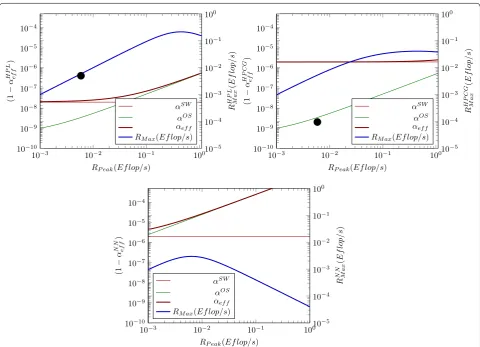
Figure 3 attempts to provide a feeling on the effect of the software contribution and of an increased clock period length. A fictive supercomputer (with behavior
somewhat similar to that of supercomputer Taihulight ) is modeled, and combined with an increased clock period length. All subfigures have dual scaling. The blue diagram line refers to the right-hand scale and shows the payload performance; all the rest to the left-hand scale and display (1−αeffXX) (for the details see [35]) contributions to the non-parallelizable fraction.
Since the behavior of the brain simulation is more similar to the “real-life” applications, the starting point to demonstrate the effect of the considerably increased clock period is the HPCG benchmark (see the top right Fig. 3). As displayed on the bottom figure, the increased clock period results in considerably higher contribution from the operating system (green line), making it domi-nant. This results in both a considerable decrease in the payload performance and shifts the peak of the payload performance toward lower nominal performance values. Notice that the performance breakdown shown in the figures were experimentally measured by [36] (Fig. 7) and [4] (Fig. 8). Because of the architectural features of the implementations (more neural processors in a com-puter core, mixing OS scheduling and time-stamped messages, changing contributions due to context switch-ing, etc.), the diagram lines describe the behavior only qualitatively. Notice, however, that the difference in the behavior manifests only at relatively high-performance values (produced with high number of cores).
6 How to overcome the issues
The discussion above explains that a huge factor of per-formance is lost because of using a “time grid” and a wrong computing stack; both are the consequence of the 70-year-old single-processor approach. As the numerical 104
105
106
107
10−7
10−6
10−5
10−2
10−1
100
Noof cores (1−αHP L
ef f )
Ef
fi
ciency
Dependence ofEHP LandEHP CGon (1−αHP L ef f ) andN
TOP5’2018.11 Summit Sierra Taihulight Tianhe-2 Piz Daint
104
105
106
107
10−7
10−6
10−5
0.2 0.5 0.8 1
No ofco
res
(1−αef f)
Ef
fi
ciency
Dependence ofEHP Lon (1−αef f) andN
Piz Daint 2012/11 2013/06 2013/11 2016/11 2017/06 2018/11
examples above demonstrate, the length of the clock period and the need for context change are in close competition for dominating the performance, but any-how they together produce a strong upper bound for the performance.
This simple qualitative analysis finds 3 orders of magni-tude of the lost performance: the (apparent) performance loss is due to the thousand times shorter execution time: the merit of the parallelism depends on the length of the measurement time. The rest can be attributed to that the simulator makes control and timing, and it takes a considerable amount of time for switching con-text and making the needed calculations; i.e., that the
present general-purpose processors cannot make a bet-ter job when imitating neurons. As it was demonstrated by [36], through organizing the threads in a more rea-sonable way, the performance of the simulators can be considerably enhanced. Those solutions, however, only influence the magnitude of the saturation and the posi-tion where it occurs: the saturation is an inherent feature of systems simulating the operation of brain on sequen-tial-parallel systems. As discussed in [43], the “general-purpose” processors are focussing on computing, rather than on interacting with each other. The importance of the cooperation is well underpinned by the fact that the processor supporting “cooperative computing” [29] kept
10−3 10−2 10−1 100
10−10
10−9
10−8
10−7
10−6
10−5
10−4
RP eak(Ef lop/s)
(1
−
α
HP
L
ef
f
)
10−5
10−4
10−3
10−2
10−1
100
R
HP
L
Ma
x
(
Ef
lo
p/
s
)
αSW
αOS
αef f
RMax(Ef lop/s)
10−3 10−2 10−1 100
10−10
10−9
10−8
10−7
10−6
10−5
10−4
RP eak(Ef lop/s)
(1
−
α
HP
CG
ef
f
)
10−5
10−4
10−3
10−2
10−1
100
R
HP
CG
Ma
x
(
Ef
lo
p/
s
)
αSW
αOS
αef f
RMax(Ef lop/s)
10−3 10−2 10−1 100
10−10
10−9
10−8
10−7
10−6
10−5
10−4
RP eak(Ef lop/s)
(1
−
α
NN ef
f
)
10−5
10−4
10−3
10−2
10−1
100
R
NN Ma
x
(
Ef
lo
p/
s
)
αSW
αOS
αef f
RMax(Ef lop/s)
Fig. 3 Contributions (1−αXeff) to (1−α total
supercomputer Taihulight in the first slot on the list of top supercomputers as well as that through optimizing internally the calculations utilizing the cooperation of the processors can considerably enhance the (apparent) com-puting performance of the supercomputer [26].
When implementing artificial neurons, more than one abstraction levels shall be introduced. At behavioral level, abstract rather than physiological parameters and less computing-intensive methods of calculations should be used. The performance can also be enhanced through introducing direct notifications and core-level (rather than system level) timing, using ideas from [29, 43]. For more details see [35]. The real solution, however, would be to renew the outdated SPA computing model [8] (when utilizing processors for simulating the brain oper-ation). Since the modeled biological objects have no cen-tral clock cycle, the other way round would be to design (from scratch) a new architecture, a biologically inspired neural network, rather than adapting system of parallel-ized processors and components based on the principles of sequential processing.
7 Summary
Simulating the inherently massively parallel brain uti-lizing inherently sequential conventional comput-ing systems is a real challenge. Accordcomput-ing to the recent studies [4, 36] both the purely SW simulation and the specially designed (but SPA processor-based) HW simu-lation currently show very similar performance limita-tions and saturation. The present paper interpreted why even the special-purpose HW simulator cannot match the performance of the human brain in real time. It was explained that the reason is the operating principle itself (or more precisely: the computing paradigm plus its tech-nical implementation together). Based on the experiences with the rigorously controlled database of supercomputer performance data, the performance of the large artificial neural networks was placed on the map of performance of the high-performance computers. The conclusion is that processor-based brain simulators using the present computing paradigms and technology surely cannot sim-ulate the whole brain (i.e., study processes like plasticity, learning, and development), and especially not in real time.
Competing interests
The authors declare that they have no competing interests.
Availability of data and materials
Not applicable. The paper used publicly available data, from publications listed in the bibliography.
Funding
Project No. 125547 has been implemented with the support provided from the National Research, Development and Innovation Fund of Hungary, financed under the K funding scheme. The funding body played no role in making the research and writing the manuscript.
Publisher’s Note
Springer Nature remains neutral with regard to jurisdictional claims in pub-lished maps and institutional affiliations.
Received: 17 January 2019 Accepted: 10 March 2019
References
1. Aspray W (1990) John von Neumann and the origins of modern comput-ing. MIT Press, Cambridge, pp 34–48
2. von Neumann J (1945) First draft of a report on the EDVAC. http://www. wiley .com/legac y/wiley chi/wang_archi /supp/appen dix_a.pdf
3. Amdahl GM (1967) Validity of the single processor approach to achieving large-scale computing capabilities. AFIPS Conf Proc 30:483–485 4. van Albada SJ et al (2018) Performance comparison of the digital
neuromorphic hardware SpiNNaker and the neural network simulation software NEST for a full-scale cortical microcircuit model. Front Neurosci 12:291
5. Hameed R, et al (2010) Understanding sources of inefficiency in general-purpose chips. In: Proceedings of the 37th annual international sympo-sium on computer architecture, ACM, New York, ISCA’10, pp 37–47 6. US National Research Council (2011) The future of computing
perfor-mance: Game over or next level? http://scien ce.energ y.gov/~/media / ascr/ascac /pdf/meeti ngs/mar11 /Yelic k.pdf
7. IEEE (2013) IEEE rebooting computing. http://reboo tingc omput ing.ieee. org/
8. Végh J (2018) Renewing computing paradigms for more efficient paral-lelization of single-threads. Advances in parallel computing, vol 29. IOS Press, Amsterdam, chap 13, pp 305–330
9. Hwang K, Jotwani N (2016) Advanced computer architecture: parallelism, scalability, programmability, 3rd edn. Mc Graw Hill, New York
10. Végh J, Vásárhelyi J, Drótos D (2019) Can parallelization save the (comput-ing) world? Adv Sci Technol Eng Syst J 4:141–158
11. Bourzac K (2017) Streching supercomputers to the limit. Nature 551:554–556
12. Denning PJ, Lewis T (2017) Exponential laws of computing growth. Com-mun ACM 60:54–65
13. Liao X et al (2018) Moving from exascale to zettascale computing: chal-lenges and techniques. Front Inf Technol Electron Eng 19(10):1236–1244 14. Markov I (2014) Limits on fundamental limits to computation. Nature
512(7513):147–154
15. Paul JM, Meyer BH (2007) Amdahl’s Law revisited for single chip systems. Int J Parallel Program 35(2):101–123
16. Dévai F (2017) The refutation of Amdahl’s Law and its variants. In: Gervasi O, Murgante B, Misra S, Borruso G, Torre CM, Rocha AMA, Taniar D, Apdu-han BO, Stankova E, Cuzzocrea A (eds) Computational science and its applications—ICCSA 2017. Springer, Cham, pp 480–493
17. Krishnaprasad S (2001) Uses and abuses of Amdahl’s Law. J Comput Sci Coll 17(2):288–293
18. Pingali K et al (2011) The tao of parallelism in algorithms. SIGPLAN Not 46(6):12–25
19. Végh J, Molnár P (2017) How to measure perfectness of parallelization in hardware/software systems. In: 18th International Carpathian control conference ICCC, pp 394–399
20. Karp AH, Flatt HP (1990) Measuring parallel processor performance. Com-mun ACM 33(5):539–543
21. Végh J (2017) Statistical considerations on limitations of supercomputers. CoRR arXiv :abs/1710.08951
23. David T, Guerraoui R, Trigonakis V (2013) Everything you always wanted to know about synchronization but were afraid to ask. In: Proceedings of the twenty-fourth ACM symposium on operating systems principles (SOSP’13), pp 33–48
24. Eyerman S, Eeckhout L (2010) Modeling critical sections in Amdahl’s Law and its implications for multicore design. SIGARCH Comput Arch News 38(3):362–370
25. Yavits L, Morad A, Ginosar R (2014) The effect of communication and synchronization on Amdahl’s law in multicore systems. Parallel Comput 40(1):1–16
26. Ao Y, Yang C, Liu F, Yin W, Jiang L, Sun Q (2018) Performance optimization of the HPCG benchmark on the Sunway TaihuLight supercomputer. ACM Trans Arch Code Optim 15(1):11:1–11:20
27. Dongarra J (2016) Report on the Sunway TaihuLight system. Technical Report UT-EECS-16-742, Department of Electrical Engineering and Com-puter Science, University of Tennessee
28. Tsafrir D (2007) The context-switch overhead inflicted by hardware inter-rupts (and the enigma of do-nothing loops). In: Proceedings of the 2007 workshop on experimental computer science, ACM, New York, ExpCS’07, p 3
29. Zheng F et al (2015) Cooperative computing techniques for a deeply fused and heterogeneous many-core processor architecture. J Comput Sci Technol 30(1):145–162
30. DeBenedictis EP (2005) Petaflops, Exaflops, and Zettaflops for science and defense. http://deben edict is.org/erik/SAND-2005/SAND2 005-2690-CUG20 05-B.pdf
31. US Government NSA and DOE (2016) A report from the NSA-DOE techni-cal meeting on high performance computing. https ://www.nitrd .gov/ nitrd group s/image s/b/b4/NSA_DOE_HPC_TechM eetin gRepo rt.pdf
32. European Commission (2016) Implementation of the action plan for the European high-performance computing strategy. http://ec.europ a.eu/ newsr oom/dae/docum ent.cfm?doc_id=15269
33. Japan Tests Silicon for Exascale Computing in 2021. (2018) https ://www. extre metec h.com/compu ting/27255 8-japan -tests -silic on-for-exasc ale-compu ting-in-2021
34. TOP500org (2016) The top 500 supercomputers. https ://www.top50 0.org/
35. Végh J (2018) Limitations of performance of exascale applications and supercomputers they are running on. ArXiv e-prints arXiv :1808.05338 36. Ippen T, Eppler JM, Plesser HE, Diesmann M (2017) Constructing neuronal
network models in massively parallel environments. Front Neuroinf 11:30 37. Rast AD, et al (2010) Scalable event-driven native parallel processing:
the SpiNNaker neuromimetic system. In: 2010 Proceedings of 7th ACM international conference on computing frontiers, pp 21–30. https ://doi. org/10.1145/17872 75.17872 79
38. HPCG Benchmark (2016) HPCG Benchmark. http://www.hpcg-bench mark.org/
39. Furber SB et al (2013) Overview of the SpiNNaker system architecture. IEEE Trans Comput 62(12):2454–2467
40. David FM, Carlyle JYC, Campbell RH (2007) Context switch overheads for Linux on ARM platforms. In: Proceedings of 2007 workshop on experi-mental computer science, Article No. 3
41. Schlansker M, Rau B (2000) EPIC: explicitly parallel instruction computing. Computer 33(2):37–45
42. Kunkel S et al (2014) Spiking network simulation code for petascale computers. Front Neuroinf 8:78