Effective hyperparameter optimization using Nelder-Mead method in deep learning

(1)

R E S E A R C H P A P E R

Open Access

Effective hyperparameter optimization

using Nelder-Mead method in deep learning

Yoshihiko Ozaki

1,2

, Masaki Yano

1,2

and Masaki Onishi

1,2*

Abstract

In deep learning, deep neural network (DNN) hyperparameters can severely affect network performance. Currently, such hyperparameters are frequently optimized by several methods, such as Bayesian optimization and the

covariance matrix adaptation evolution strategy. However, it is difficult for non-experts to employ these methods. In this paper, we adapted the simpler coordinate-search and Nelder-Mead methods to optimize hyperparameters. Several hyperparameter optimization methods were compared by configuring DNNs for character recognition and age/gender classification. Numerical results demonstrated that the Nelder-Mead method outperforms the other methods and achieves state-of-the-art accuracy for age/gender classification.

Keywords: Hyperparameter optimization, Nelder-Mead method, Deep learning, Convolutional neural network

1 Introduction

The evolution of deep neural networks (DNNs) has dra-matically improved the accuracy of character recognition [1], object recognition [2, 3], and other tasks. However, the their increasing complexity increases the number of hyperparameters, which makes tuning of hyperparame-ters an intractable task.

Traditionally, DNN hyperparameters are adjusted using manual search, grid search, or random search [4]. How-ever, search space expands exponentially relative to the number of hyperparameters; thus, such naive methods no longer work well. Therefore, more sophisticated hyperpa-rameter optimization methods are required.

In deep learning, a hyperparameter optimization prob-lem can be formulated as a stochastic black box opti-mization problem to minimize a noisy black box objective functionf(x):

Minimizef(x) (x∈χ). (1)

Here, using all information available about the objective function, we can obtain its value at pointxwith noiseas follows:

y=f(x)+, iid∼N0,σ_noise2 . (2)

*Correspondence: [email protected]

1_{Artificial Intelligence Research Center, AIST, 1-1-1 Umezono, Tsukuba, Ibaraki,} Japan

2_{University of Tsukuba, 1-1-1 Tennodai, Tsukuba, Ibaraki, Japan}

This means that no analytical properties of the objective function, e.g., its derivatives, can be optimized. In addi-tion, a loss function of the target DNN is typically chosen asf(x), and its evaluation cost is so expensive that train-ing and testtrain-ing of the DNN is required. The search space χcomprises combinations of multiple conditions such as real numbers, integers, and categories.

Currently, Bayesian optimization [5] and the covariance matrix adaptation evolution strategy (CMA-ES) [6] are considered the most promising methods for DNN hyper-parameter optimization, and their optimization ability has been proven experimentally [7–10]. However, Bayesian optimization has some hyperparameters that significantly affect its optimization performance, e.g., choices of its kernel and acquisition function. Moreover, maximizing a non-convex acquisition function is required for each iter-ation of the optimiziter-ation process. On the other hand, CMA-ES requires several populations and generations for sufficient performance. Although such calculations can be parallelized easily, significant computing resources are required.

It is evident that simple classical manual search, grid search, and random search remain common; thus, we consider that most people are unwilling to adjust the hyperparameters of a difficult optimization method or implement the method and do not have sufficient com-puting resources to optimize DNN hyperparameters.

(2)

In this paper, we describe simple substitutional ods, i.e., the coordinate-search and Nelder-Mead meth-ods, for hyperparameter optimization in deep learning. To the best of our knowledge, no report has examined the application of these methods to hyperparameter opti-mization.

Our numerical results indicate that these methods are more efficient than other well-known methods. In partic-ular, the Nelder-Mead method is the most effective for deep learning.

2 Related work

2.1 Random search

Random search is one of the simplest ways to optimize DNN hyperparameters. This method iteratively generates hyperparameter settings and evaluates the objective func-tion. Random search has excellent parallelization and can handle integer and categorical hyperparameters naturally. Bergstra and Bengio demonstrated that random search outperforms a manual search by a human expert and grid search [4].

2.2 Bayesian optimization

Bayesian optimization is one of the most remarkable hyperparameter optimization methods in recent years. Its base concept was proposed in the 1970s; however, it has been significantly improved since then due to the attention paid to DNN hyperparameter optimization.

There are several variations of Bayesian optimization, e.g., Gaussian process (GP)-based variation [11], Tree-structured Parzen Estimator (TPE) [7], and Deep Net-works for Global Optimization (DNGO) [12]. The most standard one is the GP-based variation.

GP-based Bayesian optimization is shown in

Algorithm 1. In this method, we assume that an objective

Algorithm 1:Bayesian optimization [11] fort=1, 2,. . .do

Findxtby optimizing the acquisition function over GP:xt=argmaxxu(x|D1:t−1);

Sample the objective function:yt=f(xt)+t; Augment the dataD1:t= {D1:t−1,(xt,yt)}and update the GP;

end

function follows the GP specified by its mean functionm

and kernelk:

f(x)∼GP(m(x),k(x,x)). (3)

For simplicity, we assume m(x) = 0. Then, we must consider the kernelk(x,x). For the kernel, an automatic

relevance determination (ARD) squared exponential (SE) kernel

KSE(x,x)=θ0exp

−1 2r

2₍_x,_x₎

,

wherer2(x,x)= D

d=1

xd−xd 2_/θ2

d,

(4)

or ARD Matérn 5/2 kernel

KM52(x,x)

=θ0

1+

5r2₍_x,_x₎₊5 3r

2₍_x,_x₎ _exp₋₅_r2₍_x,_x₎_,

(5)

is commonly used in Bayesian optimization [8]. Here,θ0, θ1,. . ., andθDare the kernel’s hyperparameters.

Oncek(x,x)is determined, we can predict information about a new sample pointxt+1from previous observations D1:t= {x1:t,y1:t}:

P(yt+1|D1:t,xt+1)=N

μt(xt+1),σt2(xt+1)+σnoise2

,(6)

μt(xt+1)=kT

K+σ_noise2 I−_y1

1:t, (7)

σ2

t(xt+1)=k(xt+1,xt+1)−kT

K+σ_noise2 I−1k (8)

where K=

⎡ ⎢ ⎣

k(x1,x1) · · · k(x1,xt) ..

. . .. ...

k(xt,x1) · · · k(xt,xt) ⎤ ⎥ ⎦+σ2

noiseI,

k=[k(xt+1,x1)k(xt+1,x2) · · · k(xt+1,xt)] .

The remaining problem is how to determine new sam-ple points iteratively. To determine new candidates for a sample, we generally employ an acquisition function. Here, it is necessary to select an acquisition function that achieves a good balance between exploration and exploitation based on past observations. One well-known acquisition function is expected improvement (EI):

EI(x)=

(μ(x)−f(x+))(Z)+σ(x)(Z)(σ(x)>0)

0 (σ(x)=0)(9)

whereZ= μ(x)−f(x

+₎ σ(x) , x

+₌_argmax

xi∈x1:tf(xi).

The point that maximizes the acquisition function becomes a new sample point. Although maximizing the non-convex acquisition function is difficult, the evalua-tion cost of the funcevalua-tion is considerably less than that of the original objective function. Therefore, it is easier to handle than the original problem.

Practically, Bayesian optimization is combined with ran-dom search to collect initial observation data.

(3)

2.3 Covariance matrix adaptation evolution strategy

While Bayesian optimization has been developed in the machine learning community, CMA-ES has been devel-oped in the optimization community. CMA-ES is a type of evolutionary computation that demonstrates outstand-ing performance in benchmarks as a state-of-the-art black box optimization method [13].

The (μW, λ)-CMA-ES [6] is shown in Algorithm 2. It conducts a weighted recombination from theμbest out ofλindividuals. The procedure is explained as follows.

Algorithm 2:The (μW,λ)-CMA-ES [6]

Initialize the meanx(w0), and the standard deviation σ(0)_;

pc(0)=0;pσ(0)=0;C(0)=I; forg=0, 1,. . .do

Generateg+1 generationλindividuals; Selectμbest individuals;

Update the evolution path and the covariance matrix;

Update the evolution path and the step size; end

(i) Initialize the meanx(w0)and the standard deviation σ(0)_{of individuals. Set the evolution path}

p(c0)=pσ(0)=0and the covariance matrixC(0)=I. (ii) Generateg+1generation individuals

x(_kg+1)(k=1,. . .,λ):

x(_kg+1)= x(wg)+σ(g)B(g)D(g)z(_kg+1), (10)

where

x(wg):= 1

μ

i=1wi

μ

i=1 wix(i:gλ),

B(g)D(g)B(g)D(g)T=C(g),

z(_kg+1)∼N(0,I).

Here,w1,. . .,wμare weights, andi:λdenotes thei th best individual.

(iii) Update the evolution pathp(cg)and the covariance matrixC(g):

p(cg+1)=(1−cc)p(cg)+ccucwB(g)D(g)z(wg+1), (11)

C(g+1)=(1−ccov)C(g)+ccovp(cg+1)

p(cg+1) T

, (12)

where

cu_c :=cc(2−cc),

cw:=

μ

i=1wi

_μ

i=1w2i ,

z(wg+1):= 1

μ

i=1wi

μ

i=1

wiz(i:gλ+1).

Here,ccandccovare hyperparameters.

(iv) Update the evolution pathp(σg)and the step sizeσ(g):

p(σg+1)=(1−cσ)p(σg)+cu_σcwB(g)z(wg+1), (13)

σ(g+1)₌_σ(g)_exp

1

dσ

p(σg+1)− ˆχn

ˆ χn

, (14)

where c u

σ :=

c_σ(2−c_σ), ˆ

χn=E[N(0,I)] .

Here,cσanddσ are hyperparameters.

Details about the hyperparameters used to update CMA-ES parameters are provided in the literature [6].

Since evaluations of each individual for each generation can be calculated simultaneously, CMA-ES can be paral-lelized easily. Watanabe and Le Roux and Loshchilov et al. demonstrated that CMA-ES outperforms manual search by a human expert and Bayesian optimization in certain cases [9, 10].

3 Coordinate-search and Nelder-Mead methods

In the previous section, we introduced the random search, Bayesian optimization, and CMA-ES methods. Note that the achievements of these methods have already been proven experimentally, and the results indicate that the latter two methods are very promising and considered superior to random search. However, both Bayesian optimization and CMA-ES have many hyperparameters related to their optimization performance. To set these hyperparameters appropriately, it is necessary to have suf-ficient knowledge about the given method. In addition, Bayesian optimization must maximize its non-convex acquisition function, and CMA-ES requires significant computing resources to exploit its advantages. These fac-tors make it difficult for non-experts to utilize these methods.

In this section, we introduce two optimization meth-ods, coordinate-search and Nelder-Mead, that are easy to implement. These methods have fewer hyperparameters to adjust and are practically usable with fewer computing resources.

3.1 Mathematical concepts

Before introducing the methods, we define some required mathematical concepts here.

Definition 1The positive span of a set of vectors

[v1· · ·vr]∈Rnis the convex cone:

{v∈Rn:v=α1v1+ · · · +αrvr, αi≥0, i=1,. . .,r}.

(4)

Definition 3 The set[v1· · ·vr]∈Rnis considered posi-tively dependent if one of the vectors is in the positive span of the remaining vectors; otherwise, the set is considered positively independent.

Definition 4A positive basis forRnis a positively inde-pendent set whose positive span isRn. A positive basis for

Rn_{that has n}₊₁_{vectors is considered a minimal positive} basis and a positive basis that has2n vectors is considered a maximal positive basis (Fig.1). Here, a maximal positive basis is denoted asD⊕.

Definition 5A simplex of dimension m is a con-vex hull of an affinely independent set of points Y = {y0,y1,. . .,ym}.

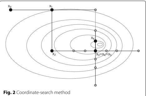
3.2 Coordinate-search method

The coordinate-search method [14] (Algorithm 3, Fig. 2) is one of the simplest direct search methods. It minimizes its objective function iteratively using the maximal positive basisD⊕=[I −I]=[e1 · · · en −e1 · · · −en].

Algorithm 3:Coordinate-search method [14] Initialization: Choosex0andα0>0; fork=0, 1,. . .do

Poll step;

Parameter update; end

This method performs a poll step iteratively to search a better solution and updates parameters to adjust its learning rate.

(i) Poll step:Order the poll setPk = {xk+αkd: d∈D⊕}. Evaluatef at the poll points in order. If a poll pointxk+αkdkthat satisfies the condition f(xk+αkdk) <f(xk)is found, then stop polling, set xk+1=xk+αkdk, and declare the iteration and poll step successful.

(ii) Parameter update:If iterationk succeeds, then set αk+1=αk(orαk+1=2αk). Otherwise, setαk+1=αk/2.

Fig. 1Maximal positive basis (D1) and minimal positive basis (D2) inR2

Fig. 2Coordinate-search method

When the step size becomes sufficiently small, the search is terminated. Note that the evaluation of functions in the poll step can be parallelized.

This method deteriorates the performance for search ranges with different scales; thus, in this study, we normal-ize parameters to [0, 1] in our computational experiments. In addition, we adopt the updating ruleαk+1 = 2αk on iteration success and order the vectors of the poll set randomly for each iteration.

3.3 Nelder-Mead method

The Nelder-Mead method [14, 15] (Algorithm 4, Fig. 3) is an optimization method that uses a simplex proposed by Nelder and Mead. Gilles et al. applied this method for the hyperparameter tuning problem in support vector machine modeling. They demonstrated that the method can find very good hyperparameter settings reliably for support vector machines [16]. Currently, the Nelder-Mead method is not considered in DNN research; however, it has a long history and many achievements in other research areas [14]. Thus, we think it is worth considering

Algorithm 4:Nelder-Mead method [15]

Initialization: Choose an initial simplex of vertices Y0=

y0₀,y1₀,. . .,yn₀. Evaluatef at the points inY0. Choose constants:

0< γs<1, −1< δic<0< δoc< δr < δe.

(5)

Fig. 3Nelder-Mead method

the Nelder-Mead method for DNN hyperparameter opti-mization. In the study by Gilles et al., their SVM has only two hyperparameters. On the other hand, DNNs often have more than 10 times number of hyperparameters. So, our task is more challenging.

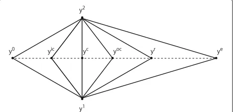
The Nelder-Mead method minimizes the objective function by repeating its evaluation at each vertex of the simplex and by replacing points according to the following procedure (Figs. 4 and 5).

(i) Order:Order then+1verticesY=y0,y1,. . .,yn as follows:

f0=f(y0)≤f1=f(y1)≤ · · · ≤fn=f(yn).

(ii) Reflect:Reflect the worst vertexynover the centroid yc=n_i₌−₀1yi/nof the remainingn vertices:

yr=yc+δr(yc−yn).

Evaluatefr=f(yr). Iff0≤fr<fn−1, then replace ynwith the reflected pointyrand terminate iteration k :Yk+1=

y0,y1,. . .,yn−1,yr. (iii) Expand:Iffr <f0, calculate:

ye=yc+δe(yc−yn)

and evaluatefe=f(ye). Iffe≤fr, then replaceyn with the expansion pointyeand terminate iteration k :Yk+1=

y0,y1,. . .,yn−1,ye. Otherwise, replace

Fig. 4Reflection, expansion, outside contraction, and inside contraction of a simplex by the Nelder-Mead method

Fig. 5Shrinking a simplex by the Nelder-Mead method.y1_and_y2_are

shrunk toys1_and_ys2_{, respectively}

ynwith the reflected pointyrand terminate iteration k :Yk+1=

y0,y1,. . .,yn−1,yr.

(iv) Contract:Iffr≥fn−1, then a contraction is performed between the best ofyrandyn.

(a) Outside contraction:Iffr <fn, perform an outside contraction:

yoc=yc+δoc(yc−yn)

and evaluatefoc=f(yoc). Iffoc≤fr, then replaceynwith the outside contraction point yoc_k and terminate iterationk :

Yk+1=

y0,y1,. . .,yn−1,yoc. Otherwise, perform a shrink.

(b) Inside contraction:Iffr_≥_fn_{, perform an} inside contraction:

yic=yc+δic(yc−yn)

and evaluatefic=f(yic). Iffic<fn, then replaceynwith the inside contraction point yicand terminate iterationk :

Yk+1= {y0,y1,. . .,yn−1,yic}. Otherwise, perform a shrink.

(v) Shrink:Evaluatef at the n points

y0+γs(yi−y0),where i=1,. . .,n, replace y1,. . .,ynwith these points, and terminate iteration k :Yk+1= {y0+γs(yi−y0), i=0,. . .,n}.

Here,γs,δic,δoc,δr, andδeare constant hyperparame-ters usually taking the following values:

γs₌ 1 2,δ

ic_{= −}1 2,δ

oc₌ 1 2,δ

r₌_{1 and}_δe₌_2. ₍₁₅₎

Note that each step of an iteration, e.g., initialization and shrink operations, can be parallelized easily.

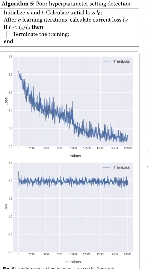
4 Poor hyperparameter setting detection

(6)

When appropriate hyperparameter values are given, train-ing loss is reduced in each iteration (Fig. 6, top graph); otherwise, regardless of how many iterations have been executed, training loss is not reduced (Fig. 6, bottom graph).

The advantage of human experts is that they can detect training failures and terminate them at an early stage. Domhan et al. proposed a method that accelerates hyper-parameter optimization methods by detecting and termi-nating such training failures using learning curve predic-tion [17]. In addipredic-tion, Klein et al. proposed a specialized Bayesian neural network to model DNN learning curves [18, 19]. We apply Algorithm 5 to detect training failures at an early stage.

Algorithm 5:Poor hyperparameter setting detection Initializenandt. Calculate initial lossl0;

Afternlearning iterations, calculate current lossln; ift<ln/l0then

Terminate the training; end

Fig. 6Learning curve when training is successful (top) and unsuccessful (bottom)

Note that this method does not optimize hyperparam-eters directly, but accelerates a hyperparameter optimiza-tion method. If a large number of training iteraoptimiza-tions with poor hyperparameter settings appear in the optimization process, this detection process improves the execution time of the optimization method.

In our experiments, we apply this method to all hyper-parameter optimization methods withnequaling 10% of the training iterations andtequaling 0.8. These values are chosen based on experience. As can be seen in Fig. 6, the learning curve of poor hyperparameter settings is distinc-tive and easy to detect; thus, there is no need to be too careful to decidenandt.

5 Numerical results

We perform computational experiments to optimize real and integer hyperparameters in combination with vari-ous datasets, tasks, and convolutional neural networks (CNNs) to compare the performance of the random search, Bayesian optimization, CMA-ES, coordinate-search, and Nelder-Mead methods.

The experimental settings for each method are given in Table 1. We use the first 100 random search evaluations to initialize the Bayesian optimization and coordinate-search methods. The number of evaluations and initial-ization parameters of CMA-ES and Bayesian optiminitial-ization are determined with reference to the literature [10]. We implement CMA-ES using Distributed Evolutionary Algo-rithms in Python (DEAP) [20], which is an evolutionary computation framework. In addition, for optimization methods that cannot handle integer values directly, inte-ger hyperparameters are handled as continuous values and rounding is performed when evaluating the objective function.

Table 1Experimental setting for each method

Method Detail

Random search Perform 600 random evaluations.

Bayesian optimization Initialize the observation data with the first 100 evaluations of the random search, then perform the optimization with exactly 500 evaluations. The kernel is the ARD Matérn 5_/2 and the acquisition function is the EI [8, 10].

CMA-ES Perform 600 evaluations with 20 generations

where each generation consists of 30 individuals.x(_w0)₌0.5,_σ(0)₌_{0.2. All} variables are scaled to [ 0, 1] [10].

Coordinate-search method

Initializex0as the best point of the first 100

random search evaluations, then perform optimization for up to 500 evaluations.

α=0.5. All variables are scaled to [ 0, 1]. Nelder-Mead method Generate an initial simplex randomly, then

perform optimization for up to 600 evaluations (including initialization).

γs₌ 1

(7)

Fig. 7MNIST database of handwritten digits [21]

5.1 MNIST

The LeNet [1] hyperparameters are optimized by the five methods to measure their performance. This network per-forms a 10-class classification of the MNIST handwritten digit database [21] (Fig. 7). Here, we use Caffe’s tutorial implementation [22, 23]. This implementation uses a rec-tified linear unit [24] as its activation function rather than the sigmoid used in the original LeNet.

These methods are also applied to the optimization of hyperparameters of the Batch-Normalized Maxout Net-work in NetNet-work proposed by Chang et al. [25]. Note that this network is deeper and has many more hyperparame-ters to optimize than LeNet.

Tables 2, 3, 4, 5, 6, and 7 show the details of each network, the fixed hyperparameters, the optimized hyper-parameters, and the search ranges. Note that prepro-cessing and augmentation of the training data are not performed.

Table 2LeNet network architecture [1]

Conv 1 Kernel size: 2, stride: 1, pad: 0

Pool 1 (MAX pooling) Kernel size: 2, stride: 2, pad: 2

FC 1

Table 3LeNet fixed parameters

Name Description

Iteration 10,000

Batch size 64

Learning rate decay policy inv (gamma=0.01, power=0.75) [29]

Table 4LeNet hyperparameters

Name Description Range

x1 Learning rate (=0.1x1) [1, 4]

x2 Momentum (=1−0.1x2) [0.5, 2]

x3 L2 weight decay [0.001, 0.01]

x∗₄ FC1 units [256, 1024]

Integer parameters are marked with∗

Table 5Network architecture of Batch-Normalized Maxout Network in Network [25]

Conv 1 Kernel size: 5, stride: 1, pad: 2, BN

MMLP 1-1 Kernel size: 1, stride: 1, pad: 0, k = 5, BN

Pool 1 (AVE pooling) Kernel size: 3, stride: 2, pad: 0, dropout

Pool 2 (AVE pooling) Kernel size: 3, stride: 2, pad: 0, dropout

Pool 3 (AVE pooling)

5.2 Age and gender classification

Gil and Tal proposed a CNN for age/gender classifica-tion [26]. In these experiments, the hyperparameters of this CNN are optimized by the five methods. This net-work consists of three convolution layers and two fully connected layers, receives an image, and outputs a gender label or an age group label. We use the implementation available on the project’s web page [27]. We test DNNs using the Adience DB [28] for the age/gender classifica-tion benchmark used in the literature [26] (Fig. 8). We divide the dataset into five sets, train the network with four sets, and test it with one set. Note that these pro-cesses require significant calculation time; thus, in the optimization process, cross validations are not performed. We perform cross validation for only the optimal solution among the optimal solutions of all methods and calculate the cross-validated accuracy for comparison with results in the literature [26].

Tables 8, 9, and 10 show the details of each network, the fixed hyperparameters, the optimized hyperparameters, and the search ranges. Note that, for this experiment, data augmentation is conducted in a single-crop manner [26].

5.3 Results

The experiments are executed for one month using 32 modern GPUs. The experimental results are given in

Table 6Fixed parameters of Batch-Normalized Maxout Network in Network

Name Description

Iteration 20,000

Batch size 100

(8)

Table 7Batch-Normalized Maxout Network in Network hyperparameters

x1 Learning rate (=0.1x1) [0.5, 2]

x2 Momentum (=1−0.1x2) [0.5, 2]

x4 Dropout 1 [0.4, 0.6]

x5 Dropout 2 [0.4, 0.6]

x6 Conv 1 initialization deviation [0.01, 0.05]

x9 MMLP 1-1 initialization deviation [0.01, 0.05]

Fig. 8Faces from the Adience benchmark for age/gender classification [28]

Tables 11, 12, 13, and 14. In all experiments, the Nelder-Mead method achieves both minimal loss and variance. The small variance suggests that the initial values of the method do not significantly affect the results. Fur-thermore, the accuracy of the cross validation with the best solution found by the Nelder-Mead method in gen-der classification is 87.20% (±1.328024) and that for

Table 8Network architecture of the age/gender classification CNN [26]

FC 1 Dropout

FC 2 Dropout

FC 3

Table 9Fixed parameters of the age/gender classification CNN

Name Description

Iteration 20,000

Batch size 50

Learning rate decay policy Step (gamma=0.1, step size=10000) [29]

age classification is 51.25% (±5.461970). These val-ues are higher than previous state-of-the-art results (86.8%(±1.4)and 50.7%(±5.1)) reported in the literature [26]. The stability and search performance of this method are magnificent.

The coordinate-search method also achieves good results with LeNet and Batch-Normalized Maxout Network in Network. However, the coordinate-search method searches points using each vector of the pos-itive basis; thus, convergence speed is reduced as the number of dimensions increases. This appears to be the reason why the coordinate-search method does not work for the age/gender classification CNN, which has more

Table 10Hyperparameters of the age/gender classification CNN

x1 Learning rate (=0.1x1) [1, 4]

x2 Momentum (=1−0.1x2) [0.5, 2]

x4 Dropout 1 [0.4, 0.6]

x5 Dropout 2 [0.4, 0.6]

x∗₆ FC 1 units [512, 1024]

x∗₇ FC 2 units [256, 512]

x11 FC 1 initialization deviation [0.001, 0.01]

x14 Conv 1 bias [0, 1]

x17 FC 1 bias [0, 1]

x18 FC 2 bias [0, 1]

x∗₁₉ Normalization 1 localsize₍₌2x19+3) [0, 2]

x∗₂₀ Normalization 2 localsize₍₌2x20+3) [0, 2]

x21 Normalization 1 alpha [0.0001, 0.0002]

x22 Normalization 2 alpha [0.0001, 0.0002]

x23 Normalization 1 beta [0.5, 0.95]

x24 Normalization 2 beta [0.5, 0.95]

(9)

Table 11MNIST results (LeNet)

Method Mean loss Min loss

Random search 0.005411(±0.001413) 0.002781

Bayesian optimization 0.004217(±0.002242) 0.000089

CMA-ES 0.000926(±0.001420) 0.000047

Coordinate-search method 0.000052(±0.000094) 0.000002

Nelder-Mead method 0.000029 (±0.000029) 0.000004

Method Mean accuracy (%) Accuracy with

min loss (%)

Random search 98.98(±0.08) 99.06

CMA-ES 99.20(±0.08) 99.30

The coordinate-search method 99.26(±0.05) 99.35

The Nelder-Mead method 99.24(±0.04) 99.28

The smallest loss for each experiment is indicated by bold-faced font

hyperparameters. Thus, we should use the Nelder-Mead method rather than the coordinate-search method. As demonstrated in the literature [9], CMA-ES is superior to random search because it finds better parameters ear-lier. Despite using the same hyperparameters for Bayesian optimization, the method works well for age estimation but not for other tasks. This indicates that, for Bayesian optimization, hyperparameters should be adjusted care-fully depending on the given task.

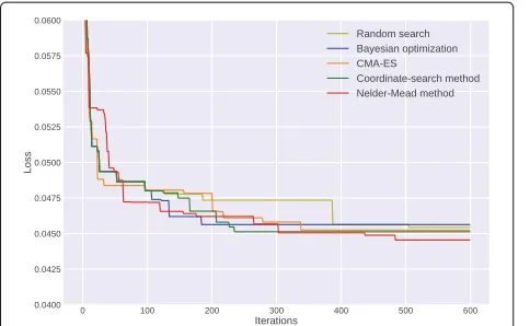
The mean loss graphs (Figs. 9, 10, 11 and 12) show that the Nelder-Mead method rapidly finds a good solu-tion and converges faster than the other methods. We anticipate that the objective function for hyperparame-ter optimization is multimodal, and many local optima that achieve similar results exist. We confirmed this property via additional experiments that optimized the

Table 12MNIST Results (Batch-Normalized Maxout Network in Network)

Random search 0.045438₍_±0.002142₎ 0.042694

CMA-ES 0.045248(±0.002537) 0.042250

Coordinate-search method 0.045131(±0.001088) 0.043639

Nelder-Mead method 0.044549 (±0.001079) 0.043238

min loss (%)

Random search 99.56₍_±0.02₎ 99.58

CMA-ES 99.49(±0.14) 99.59

Nelder-Mead method 99.53(±0.00) 99.54

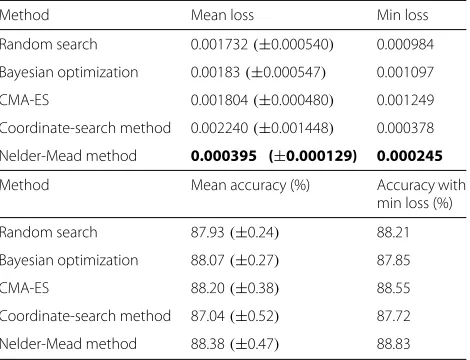
Table 13Gender classification results

Random search 0.001732₍_±0.000540₎ 0.000984

CMA-ES 0.001804(±0.000480) 0.001249

Nelder-Mead method 0.000395 (±0.000129) 0.000245

min loss (%)

Random search 87.93₍_±0.24₎ 88.21

CMA-ES 88.20(±0.38) 88.55

hyperparameters of the gender classification CNN, the network which has the largest search space, using the Nelder-Mead method. The optimized hyperparameter settings after 600 evaluations of each experiment are shown using the parallel coordinates plot in Fig. 13. In the figure, points in the search space are represented as polylines with vertices on parallel axes. The position of the vertex on theith axis corresponds to the value of the hyperparameterxi. The polylines exhibiting small losses are shown in dark colors.

Experimental results showed that the Nelder-Mead method converged to different points every time and the objective function was almost multimodal. Differ-ent hyperparameters settings achieved similar losses. From Table 13 and Fig. 13, we deduce that many local optima that achieve similar results exist. In such cases,

Table 14Age classification results

Random search 0.035694₍_±0.006958₎ 0.026563

CMA-ES 0.031244(±0.010834) 0.016952

Nelder-Mead method 0.015492 (±0.002276) 0.013556

min loss (%)

Random search 57.18₍_±0.96₎ 57.90

CMA-ES 57.17(±0.80) 58.19

(10)

Fig. 9Mean loss of all executions for each method per iteration (LeNet)

the Nelder-Mead method tends to directly converge to a close local optimum without being influenced by the objective function values of distant points. In contrast, other methods perform a global search, e.g., Bayesian optimization and CMA-ES try to find potential candi-dates of global optima and require more iterations to find a local optimum in comparison to the Nelder-Mead method.

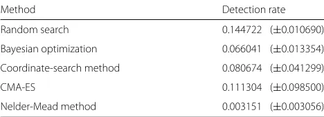
According to the poor hyperparameter setting detection rates (Tables 15, 16, 17, and 18), on average, approxi-mately 8, 1, 33, and 26% of executions in each experiment are detected as having poor hyperparameter settings and optimization is accelerated in proportion to the detec-tion rate. In particular, the CNN for age/gender clas-sification tends to be very sensitive to hyperparameter settings.

Note that the Nelder-Mead method rarely generates poor hyperparameter settings because of its strategy, e.g., reflection moves the simplex in a direction away from the point of poor hyperparameter settings.

Fig. 10Mean loss of all executions for each method per iteration (Batch-Normalized Maxout Network in Network)

Fig. 11Mean loss of all executions for each method per iteration (gender classification CNN)

From the above results, we conclude that the Nelder-Mead method is the best choice for DNN hyperparameter optimization.

6 Conclusions

In this study, we tested methods for DNN hyperparameter optimization. We showed that the Nelder-Mead method achieved good results in all experiments. Moreover, we achieved state-of-the-art accuracy with age/gender classification using the Adience DB by optimizing the CNN hyperparameters proposed in [26].

Complicated hyperparameter optimization methods are difficult to implement and have sensitive hyperparam-eters, which affects their performance. Therefore, it is difficult for non-experts to use these methods. In contrast, the Nelder-Mead method is easy to use and outperforms such complicated methods in many cases.

In our experiments, we optimized the hyperparameters of DNNs for character recognition and age/gender clas-sification. These tasks are important and have been well

(11)

Fig. 13Parallel coordinates plot of the optimized hyperparameters of the gender classification CNN

Table 15Poor hyperparameter setting detection rate for each method (LeNet)

Method Detection rate

Random search 0.144722 (±0.010690)

Bayesian optimization 0.066041 (±0.013354)

Coordinate-search method 0.080674 (±0.041299)

CMA-ES 0.111304 (±0.098500)

Nelder-Mead method 0.003151 (±0.003056)

Table 16Poor hyperparameter setting detection rate for each method (Batch-Normalized Maxout Network in Network)

Random search 0 (±0)

CMA-ES 0 (±0)

Nelder-Mead method 0 (±0)

known for a long time. However, it is desirable to evaluate the proposed method using the generic object recogni-tion data set. Therefore, in future, we plan to evaluate the proposed method using other data sets. A detailed analysis of the dependency on initial parameters and the

Table 17Poor hyperparameter setting detection rate for each method (gender classification CNN)

Random search 0.506177 (±0.015931)

CMA-ES 0.360734 (±0.091648)

Table 18Poor hyperparameter setting detection rate for each method (age classification CNN)

Random search 0.444667 (±0.039355)

CMA-ES 0.317533 (±0.207479)

optimization of categorical variables will be also the focus of future work.

Acknowledgements

This paper is based on results obtained from a project commissioned by the New Energy and Industrial Technology Development Organization (NEDO).

Authors’ contributions

YO implemented the hyperparameter optimization methods for DNNs, performed the experiments, and drafted the manuscript. MY implemented the hyperparameter optimization methods for DNNs and helped perform the experiments and draft the manuscript. MO guided the work, supervised the experimental design, and helped draft the manuscript. All authors have read and approved the final manuscript.

Competing interests

The authors declare that they have no competing interests.

Publisher’s Note

Springer Nature remains neutral with regard to jurisdictional claims in published maps and institutional affiliations.

Received: 9 January 2017 Accepted: 4 September 2017

References

1. LeCun Y, Bottou L, Bengio Y, Patrick H (1998) Gradient-based learning applied to document recognition. Proc IEEE 86(11):2278–2324 2. Krizhevsky A, Sutskever I, Hinton GE (2012) Imagenet classification with

deep convolutional neural networks. Adv Neural Inf Process Syst (NIPS) 25:1097–1105

(12)

4. Bergstra J, Bengio Y (2012) Random search for hyper-parameter optimization. J Mach Learn Res 13:281–305

5. Mockus J (1974) On Bayesian Methods for Seeking the Extremum. In: Optimization Techniques IFIP Technical Conference. pp 400–404 6. Hansen N, Ostermeier A (2001) Completely derandomized self-adaptation

in evolution strategies. Evol Comput 9:159–195

7. Bergstra J, Bardenet R, Bengio Y, Kégl B (2011) Algorithms for hyper-parameter optimization. Adv Neural Inf Process Syst (NIPS) 24:2546–2554

8. Snoek J, Larochelle H, Adams RP (2012) Practical Bayesian optimization of machine learning algorithms. Adv Neural Inf Process Syst (NIPS) 25:2951–2959

9. Watanabe S, Le Roux J (2014) A black box optimization for automatic speech recognition. In: International Conference on Acoustics, Speech, and Signal Processing. (ICASSP). pp 3256–3260

10. Loshchilov I, Hutter F (2016) CMA-ES for hyperparameter optimization of deep neural networks. https://arxiv.org/abs/1604.07269.

Accessed 20 Sept 2017

11. Brochu E, Cora VM, De Freitas N (2010) A tutorial on Bayesian optimization of expensive cost functions, with application to active user modeling and hierarchical reinforcement learning. https://arxiv.org/abs/1012.2599. Accessed 20 Sept 2017

12. Snoek J, Rippel O, Swersky K, Kiros R, Satish N, Sundaram N, Patwary M, Prabhat M, Adams R (2015) Scalable Bayesian optimization using deep neural networks. In: International Conference on Machine Learning. (ICML). pp 2171–2180

13. Hansen N, Auger A, Ros R, Finck S, Pošík P (2010) Comparing results of 31 algorithms from the black-box optimization benchmarking BBOB-2009. In: Proceedings of the 12th Annual Conference Companion on Genetic and Evolutionary Computation. pp 1689–1696

14. Conn AR, Scheinberg K, Vicente LN (2009) Introduction to derivative-free optimization. MPS-SIAM Ser Optim. http://epubs.siam.org/doi/book/10. 1137/1.9780898718768

15. Nelder JA, Mead RA (1965) Simplex method for function minimization. Comput J 7:308–313

16. Gilles C, Patrick R, Mélanie H (2005) Model selection for support vector classifiers via direct simplex search. The Florida Artificial Intelligence Research Society (FLAIRS) Conference:431–435

17. Domhan T, Springenberg JT, Hutter F (2015) Speeding up automatic hyperparameter optimization of deep neural networks by extrapolation of learning curves. In: Proceedings of the 24th International Joint Conference on Artificial Intelligence. (IJCAI). pp 3460–3468 18. Klein A, Falkner S, Springenberg JT, Hutter F (2016) Bayesian neural

networks for predicting learning curves. Workshop on Bayesian Deep Learning, NIPS. http://bayesiandeeplearning.org/2016/papers/BDL_38. pdf

19. Klein A, Falkner S, Springenberg JT, Hutter F (2017) Learning curve prediction with bayesian neural networks. International Conference on Learning Representations (ICLR). http://www.iclr.cc/doku.php?id= iclr2017:conference_posters#tuesday_morning

20. De Rainville FM, Fortin FA, Gardner MA, Parizeau M, Gagné C (2012) “DEAP: A Python Framework for Evolutionary Algorithms”. In: EvoSoft Workshop, Companion proc. of the Genetic and Evolutionary Computation Conference (GECCO). https://dl.acm.org/citation.cfm?id=2330799 21. LeCun Y, Cortes C (2010) MNIST handwritten digit database. http://yann.

lecun.com/exdb/mnist/. Accessed 20 Sept 2017

22. Yangqing J, Evan S, Jeff D, Sergey K, Jonathan L, Ross G, Sergio G, Trevor D (2014) Caffe: Convolutional architecture for fast feature embedding. https://arxiv.org/abs/1408.5093. Accessed 20 Sept 2017

23. Evan S (2014) Training LeNet on MNIST with Caffe. http://caffe. berkeleyvision.org/gathered/examples/mnist.html. Accessed 20 Sept 2017

24. Nair V, Hinton GE (2010) Rectified linear units improve restricted Boltzmann machines. International Conference on Machine Learning. https://dl.acm.org/citation.cfm?id=3104425

25. Chang JR, Chen YS (2015) Batch-Normalized Maxout Network in Network. In: Proceedings of the 33rd International Conference on Machine Learning. https://arxiv.org/abs/1511.02583. Accessed 20 Sept 2017 26. Gil L, Tal H (2015) Age and gender classification using convolutional

neural networks. Computer Vision and Pattern Recognition Workshops (CVPRW). http://ieeexplore.ieee.org/document/7301352/

27. Gil L, Tal H (2015) Age and gender classification using convolutional neural networks. http://www.openu.ac.il/home/hassner/projects/cnn_ agegender. Accessed 20 Sept 2017

28. Eran E, Roee E, Tal E (2014) Age and gender estimation of unfiltered faces. IEEE Trans Inf Forensic Secur 9(12):2170–2179