Growth, inequality and poverty dynamics
in Mexico
Alberto Javier Iniguez‑Montiel
1*and Takashi Kurosaki
21 Introduction
This study investigates the contribution of both growth and redistribution to pov-erty reduction in Mexico during the period from 1992 to 2014. Moreover, by control-ling for the potential bias due to intertemporal changes in the official poverty lines and the spurious correlation bias that can occur if the same microdata are used to gener-ate measures of growth, inequality, and poverty, this study intends to shed new light on the dynamic relationships that exist between growth, inequality and poverty in Mexico. This study thus helps validating important and hotly debated hypotheses in development economics.
In the development economics literature, there is a general consensus that growth is good for the poor (Besley and Burgues 2004; Dollar and Kraay 2002) and that a reduc-tion in inequality contributes to a decline in poverty (Bourguignon 2004; Dagdeviren
Abstract
In this study, we examine the contributions of growth and redistribution to poverty reduction in Mexico during the period from 1992 to 2014, using repeated cross‑section household data. We first decompose the observed changes in poverty reduction into components arising from growth, improved income distribution, and heterogeneous inflation. We find the component of inflation to be non‑negligible and highly detri‑ mental to the poor, as the inflation experienced by them has been higher than the national average since 2008. The decomposition also shows improvement in income distribution to be the main contributor to poverty reduction in Mexico. In the second part of our analysis, we compile a unique panel dataset at the state level from the household data and estimate a system of equations that characterize the dynamic relationship between growth, inequality, and poverty, being careful to avoid spuri‑ ous correlation arising from data construction. The GMM regression results show that Mexican states are characterized by income and inequality convergence, that lower levels of inequality tend to spur growth in the economy, that increasing income/con‑ sumption levels contribute to reducing inequality, and that poverty reduction is highly determined by inequality levels in the previous period. This implies that once a small perturbation occurs in a state that improves the distribution of income, the state is expected to experience sustained income growth and accelerated poverty reduction simultaneously in subsequent periods.
Keywords: Dynamics, GMM estimation, Growth, Inequality, Poverty, Mexico JEL classification codes: C23, I32, O15, O47, O54
Open Access
© The Author(s) 2018. This article is distributed under the terms of the Creative Commons Attribution 4.0 International License
(http://creat iveco mmons .org/licen ses/by/4.0/), which permits unrestricted use, distribution, and reproduction in any medium,
provided you give appropriate credit to the original author(s) and the source, provide a link to the Creative Commons license, and indicate if changes were made.
RESEARCH
*Correspondence: iniguez@e.u‑tokyo.ac.jp
1 Graduate School
of Economics, The University of Tokyo, 7‑3‑1 Hongo, Bunkyo, Tokyo 113‑0033, Japan
et al. 2004; Lopez 2006; Ravallion 1997, 2005). However, some have shown that not all the benefits arising from growth trickle down to the poor (Datt and Ravallion 1992; Kak-wani et al. 2000; Oxfam 2000). Furthermore, there is no guarantee that any improve-ment in the distribution of income raises the incomes of the poor (Iniguez-Montiel
2014). These issues have been hotly debated over the past decades (Jain 1990; Kakwani and Subbarao 1990; Kakwani et al. 2000; Kalwiji and Verschoor 2007; Lopez and Serven
2006; Ravallion 2001, 2007), particularly after the general agreement on the Millennium Development Goals (United Nations 2000), which embrace the ideology of a world free of poverty and hunger.
Nevertheless, several important considerations have been either overlooked or downplayed, when analyzing the particular stories of individual countries. This study addresses two of these considerations. First, most studies consider the poverty line as being constant over time, and evaluate only the impact of real growth (growth at con-stant prices) on poverty, as this is the standard treatment in the intertemporal analysis of poverty (see, for example, Deaton 1997; Ravallion 1992). However, it is possible that the official poverty lines correspond to different levels of purchasing power over time, partly due to measurement errors, heterogeneous increases in the prices of goods that com-pound the basic-needs basket for the poor, and/or changes in the social notions of abso-lute poverty over time. To address this possibility, a “triple” decomposition of poverty change has been proposed by Günther and Grimm (2007). We apply their methodology to the case of Mexico to provide a more precise overview of the relationship between poverty, inequality, and economic growth in this country. Although this methodology uses the distribution-neutral growth or zero-growth-Lorenz-curve changes as a bench-mark for the simulation exercises, it offers a clear picture of the manner in which growth, redistribution, and inflation interact dynamically, affecting poverty and the entire distri-bution of income or consumption.
Second, most of the existing studies on the relationship between growth, inequality and poverty use the three measures compiled from the microdata of household income and expenditure surveys of the same year. When a household expenditure survey dataset is available, we can aggregate the data to compile empirical variables for mean consump-tion/income, poverty, and inequality. Since the three variables in any given period are dependent by construction, regressing one on the others causes a potential bias due to spurious correlation. Such regression analyses could be valid as a mere description of the distribution of individual-level consumption/income. However, it is difficult to infer the structural relationship between growth, inequality, and poverty from these exer-cises since the changes in poverty, average income, and inequality in the same period are linked by data construction. To avoid this spurious correlation, a regional panel data analysis, using a system of equations that carefully incorporates a lagged structure, was proposed by Kurita and Kurosaki (2011). We apply their methodology to the case of Mexico using “state” within Mexico as the unit of observation.
the consistent decline of inequality observed after 2000 (Cortés 2013), particularly in the rural sector, whereas the factor that has continuously acted in the opposite direction, putting a strong break to the reduction effort and holding poverty at almost the same level as that in 1992, was the increase in food prices facing the poor since 2008.
In the second methodology, we aggregate the microdata into a unique panel dataset at the state level to estimate a system of equations, which characterizes the dynamic rela-tionship between growth, inequality and poverty in Mexico, by the generalized method of moments (GMM). We show that the parametrically estimated response from the sec-ond methodology is useful for understanding the decomposition results from the first methodology, and also for testing the validity of the relevant hypotheses for the case of Mexico. The GMM regression results indicate that Mexican states are characterized by income convergence and inequality convergence, that lower levels of inequality spur growth in the economy, that increasing income/consumption levels contribute to reduc-ing inequality, and that poverty reduction in Mexican states is highly determined by inequality levels in the previous period. Growth is also found to be poverty reducing; however, the growth elasticity of poverty is about half the size of the inequality elasticity of poverty. All our results are highly robust, deepening our understanding of the rela-tionship between poverty, inequality, and economic growth in Mexico.
There are some relevant works in the recent literature that are related to our study and that deserve our early attention. First, the important contribution of Ros (2015), who discusses in detail the causes of low economic growth and high levels of inequality in Mexico, arguing that the Mexican economy has been trapped in a low-growth-level equilibrium during the last three decades, a situation in which low growth interacts with its determinants to maintain the stability of the same pervasive equilibrium. Moreover, Ros (2015) highlights the particular relationship that exists between growth and inequal-ity in Mexico, where high levels of inequalinequal-ity contribute to reducing growth and low growth levels cause a higher concentration of income. According to our GMM results, this is indeed the case, and the benefits of a more equal distribution of income could be sizable for both the poor and non-poor alike because poverty would decline and over-all income/consumption would increase simultaneously, thus reducing the poverty level further, as implied by the sizes and signs of our estimated coefficients.
Another important work is the one of Hernández-Laos and Benítez-Lino (2014), who analyze the impact of the economic cycle on food poverty in Mexico, determining how the performance of the labor market affected the level of poverty during 2005–2012 by also estimating a system of equations at the state level by the GMM approach. Their results actually complement ours by identifying two important labor-market mecha-nisms that affect food poverty along the economic cycle, namely overall unemployment and lagged informal-sector employment with estimated elasticities of 0.06 and 0.08, respectively. It is important to mention that we also draw from their analysis to be able to provide strong evidence of the reliability of our estimates due to the non-representa-tiveness of the data at the state level. Indeed, our estimates are highly robust even when using the state-level representative data of the Mexican labor market as proposed in Hernández-Laos and Benítez-Lino (2014).
methodology suffers from several drawbacks. It should be mentioned that the main results and conclusions drawn in Millán (2014) are not supported by ours, using either the decomposition methodology of Günther and Grimm (2007) or the parametric meth-odology of Kurita and Kurosaki (2011). Particularly, Millán argues that there is always a trade-off between growth and redistribution so that each time there is an economic recession, growth increases poverty and inequality decreases it, while exactly the oppo-site effects occur each time the economy expands; therefore, inequality must be poverty augmenting during growth spells (Millán 2014). As shown consistently in our study as well as in Campos-Vázquez and Monroy (2016), such a systematic trade-off is not an economic regularity in Mexico. Everything depends on how the distribution of income changes during economic expansions or recessions as suggested in the literature (Raval-lion 2001; Lopez 2006; Cortés 2010). Therefore, our study does support a cooperative interaction between growth and inequality for/against the reduction of poverty such as the ones that occurred in Mexico during 1992–2006, 2000–2008, or 2006–2008.
The rest of the paper is organized as follows. Section 2 describes the datasets and macroeconomic background. Section 3 presents the empirical model and results using the triple decomposition applied to household-level data, and Sect. 4 discusses briefly the theories that support the system of equations to be estimated before presenting the empirical model and results using the state-level panel data. Finally, Sect. 5 concludes.
2 Data
The datasets used in this study are compiled from the Household Income and Expendi-ture Survey (ENIGH) for the period 1992–2014. The ENIGH is a nationally represent-ative survey that covers both the rural and urban populations. It has been conducted biannually since 1992 by the National Institute of Statistics, Geography and Informat-ics (INEGI) in Mexico. In addition to the biannual surveys, a similar survey was con-ducted in 2005 as well. We thus have 12 yearly observations (1992, 1994, 1996, 1998, 2000, 2002, 2004, 2005, 2006, 2008, 2010, 2012, and 2014). From these datasets, house-hold-level income figures are obtained as repeated cross sections to be used in Sect. 3
(10,530 sample households in 1992, 30,169 in 2010, and 19,479 in 2014). From these datasets, state-level average consumption/income, inequality, and poverty are compiled and used in Sect. 4. The number of states in Mexico is 32 and has not changed over time. As the time interval was different, the 2005 survey data were not used in the regression analysis. Therefore, the state-level panel dataset is balanced (32 states times 12 biannual observations).
To convert nominal figures into real figures, we followed the methodology proposed by the Technical Committee for the Measurement of Poverty (CTMP 2002) in Mexico, using the national consumer price index (CPI) and setting the data into constant prices of August 2011. The same methodology and data are used by the National Council for the Evaluation of Social Development Policy (CONEVAL) in Mexico to evaluate poverty, inequality, and other development issues as mandated by Mexican law.
official poverty lines designated by the Government of Mexico. There are three types of official poverty lines: “food,” “extreme,” and “basic-needs” (Iniguez-Montiel 2014). The food poverty line is the lowest of the three, and it is calculated as the cost of a basic-food basket for the poor to survive; the extreme poverty line additionally considers educa-tion and health necessities; the basic-needs poverty line is the highest as it covers the costs of three additional commodities/services (clothing, housing, and transportation) that are not included in the other two poverty lines. Although these official poverty lines are meant to capture the absolute poverty level that is constant over time, in reality, their purchasing powers changed over time, because of higher inflation rates for the goods that were considered to estimate the official poverty lines, compared to the goods that were included in the basket used to estimate the CPI in Mexico. In other words, the poor in Mexico suffered from inflation rates that were higher than those indicated by the national CPI. This is the reason we apply the triple decomposition methodology pro-posed by Günther and Grimm (2007).
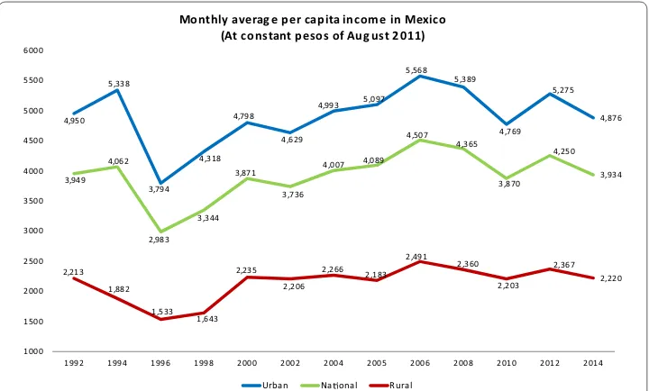
During the past three decades, which include the period covered by our datasets, the Mexican economy has grown quite slowly (Arias 2010; OECD 2009), characterized by economic instability or volatility, accompanied by several spans of negative growth rates (Iniguez-Montiel 2014). The economy grew at an annual rate of 1.07% for the period 1980–2014, or 1.82% for the period 1992–2014 in per-capita terms (Feenstra et al. 2015). According to the ENIGH, rural per-capita incomes grew by only 0.32%, whereas urban per-capita incomes shrank by 0.38% during the period 1992–2014, rendering an overall fall in average per-capita income of about 1.5% (see Fig. 1).1 This phenomenon has been
4,950 5,338
3,794 4,318
4,798
4,629
4,993 5,097
5,568 5,389
4,769 5,275
4,876
3,949 4,062
2,983 3,344
3,871
3,736
4,007 4,089
4,507 4,365
3,870 4,250
3,934
2,213 1,882
1,533 1,643
2,235 2,206
2,266 2,183
2,491 2,360
2,203 2,367
2,220
1000 1500 2000 2500 3000 3500 4000 4500 5000 5500 6000
1992 1994 1996 1998 2000 2002 2004 2005 2006 2008 2010 2012 2014
Monthly averag e per capita income in Mexico (At constant pesos of Aug ust 2011)
Urban Na onal Rural
Fig. 1 Monthly average per capita income in Mexico (at constant pesos of August 2011)
already pointed out by CONEVAL and is consistent with other labor-market indicators as well (CONEVAL 2015).
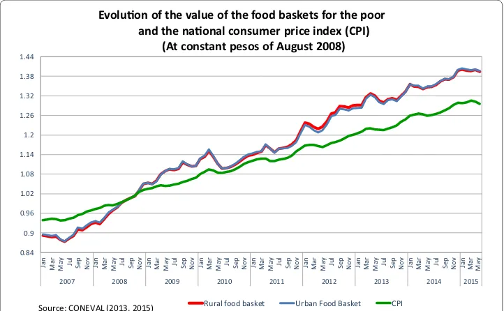
On the other hand, we can also verify that the real values of the official poverty lines (at constant prices) increased by 12% in both the rural and urban centers over the period 1992–2014.2 This implies that the price increases of goods for the poor were greater than
those faced by the nation as a whole. In other words, the purchasing power of the poor in Mexico decreased more rapidly over time than that of average Mexicans. Therefore, if we adjust real incomes in Mexico to the inflation rate underlying the poverty line, we end up with income growth rates that are actually negative. We were able to corroborate all this information in the 2012 CONEVAL’s Report of the Evolution of Social Develop-ment Policy in Mexico (CONEVAL 2013, pp 22–23), where it is clearly explained and shown that the main reason for the differential evolution of price levels between the offi-cial poverty lines and the CPI has been the continuous rise in the prices of food since 2008. Figure 2 shows this phenomenon in Mexico, from January 2007 to May 2015, by plotting the evolution of the value of the food baskets for the poor in the rural and urban areas, as well as that of the CPI, all at constant prices of August 2008. It is possible to see in the figure that, after September 2008, the rate at which food prices increase for the poor has been much faster than the inflation rate for the country as a whole and the wid-ening gaps between these indicators have been evidently worswid-ening since January 2012.
0.84 0.9 0.96 1.02 1.08 1.14 1.2 1.26 1.32 1.38 1.44 Ja n Ma r Ma
y Jul Sep
No v Ja n Ma r Ma
y Jul Sep
No v Ja n Ma r Ma
y Jul Sep
No v Ja n Ma r Ma
y Jul Sep
No v Ja n Ma r Ma
y Jul Sep
No v Ja n Ma r Ma
y Jul Sep
No v Ja n Ma r Ma
y Jul Sep
No v Ja n Ma r Ma
y Jul Sep
No v Ja n Ma r Ma y
2007 2008 2009 2010 2011 2012 2013 2014 2015
Evoluon of the value of the food baskets for the poor and the naonal consumer price index (CPI)
(At constant pesos of August 2008)
Rural food basket Urban Food Basket CPI
Source: CONEVAL (2013, 2015)
Fig. 2 Evolution of the value of the food baskets for the poor and the national consumer price index (CPI) (at constant pesos of August 2008)
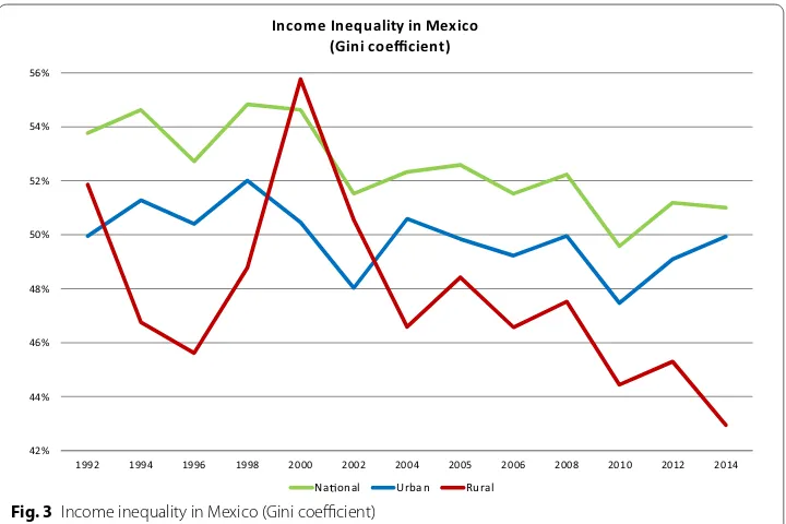
Another important characteristic of our datasets is that inequality in the distribu-tion of income declined in the country (see Fig. 3) as documented in Cortés (2013).3 For
instance, rural income inequality measured by the Gini coefficient declined by more than 6 and 9 percentage points during the periods 1992–2012 and 1992–2014, respectively, whereas urban inequality fell by 1 percentage point and remained unchanged, respec-tively, during the same periods. The impressive decline of inequality observed in the rural areas is what actually rendered the slow growth of the Mexican economy as being pro-poor (Iniguez-Montiel 2014), and which, according to our estimations, increased the incomes of the poor (those below the 50th percentile of the distribution) in the rural sector by 13% in the period 1992–2014.4 A closer examination of Fig. 3 shows that the
decline in inequality levels occurred sometime during 2000–2004 in both sectors, con-tinuing its declining trend from 2008 onwards only in the rural sector. According to the literature (Iniguez-Montiel 2011; Lustig et al. 2013), the inequality decline in Mexico after 2000 was mainly associated with a narrowing of the skill-premium gap between low- and high-skilled workers, an improvement in the distribution of education, and an increase in public transfers primarily related to redistributive polices of the 1990s and 2000s, such as Oportunidades (a conditional cash transfer program that investments in the human capital of the poor) and the Popular Health Insurance (PHI) program.
42% 44% 46% 48% 50% 52% 54% 56%
1992 1994 1996 1998 2000 2002 2004 2005 2006 2008 2010 2012 2014
Income Inequality in Mexico (Gini coefficient)
Na onal Urban Rural
Fig. 3 Income inequality in Mexico (Gini coefficient)
Progresa, the forerunner of Oportunidades, was formally initiated in 1998 and greatly expanded in 2001, whereas the PHI program was launched in 2004.
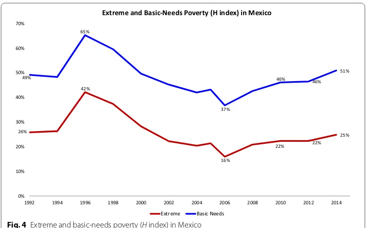
To summarize the macroeconomic situations underlying our datasets, we might say that 30 years of economic reforms and policies, since Mexico became an open econ-omy, have been completely insufficient for spurring economic growth, and that the low growth that has occurred cannot cope with the constant increase in the population as well as in the prices of goods over time. Consequently, extreme poverty was found to decline by only 1 percentage point (from 26 to 25%), whereas basic-needs poverty actu-ally increased from 49 to 51% during the period of analysis (see Fig. 4). As corroborated in the next section, the decline of extreme poverty could be mainly attributed to the lower levels of inequality in the country, especially those observed in the rural areas, where poverty has been reduced regardless of the poverty line that is used. However, poverty is persistent in the urban areas, where inequality remains high (Gini of 50%, similar to the 1992 level), and has increased because of higher levels of inflation and lower levels of income over time. It is possible that if Mexico had not adopted its main redistributive polices, poverty at all levels would have been much higher today than it was 22 years ago. These issues will be investigated in detail in the next two sections.
3 Triple decomposition of the change in poverty
3.1 Empirical methodology
Following Günther and Grimm (2007), we decompose the change in poverty measure into components arising from growth, distribution, and inflation. The method of decom-position is as follows:
�Pt+n,t=[P(µt+n,Lt,zt)−P(µt,Lt,zt)]+[P(µt,Lt+n,zt)−P(µt,Lt,zt)]
+[P(µt,Lt,zt+n)−P(µt,Lt,zt)]+Rt+n,t,
26%
42%
16%
22% 22%
25% 49%
65%
37%
46% 46%
51%
0% 10% 20% 30% 40% 50% 60% 70%
1992 1994 1996 1998 2000 2002 2004 2006 2008 2010 2012 2014
Extreme and Basic-Needs Poverty (H index) in Mexico
Extreme Basic Needs
where P(µt,Lt,zt) is the poverty measure with a mean income µt , a Lorenz curve Lt , and a poverty line zt in period t. Both µt and zt are in real terms adjusted by the national CPI in period t. The first component of the equation corresponds to the change in poverty as explained by general growth and should be interpreted as the poverty change that would have occurred with the observed growth rate, given that the poor had experienced the same increase in cost of living as indicated by the national CPI (Günther and Grimm
2007). The second component corresponds to the change in poverty as explained by the distribution effect in a growth- and poverty-line-neutral case, whereas the third com-ponent corresponds to the change in poverty as explained by the inflation difference between the poverty line and the national CPI in a growth- and distribution-neutral case.
3.2 Empirical results
We decompose poverty changes in Mexico for two periods (1992–2014 and 1992– 2010),5 the three official poverty lines (food, extreme, and basic-needs), and the three
commonly used FGT poverty measures (headcount (H), poverty gap (PG), and squared poverty gap (SPG)). The reason to consider two separate but almost identical periods is that the decomposition results are highly sensitive to the choice of periods given that the income growth that occurred in each period is remarkably different, and therefore its impact on poverty changed considerably, reflecting its high variability as described in the previous section.
3.2.1 1992–2014
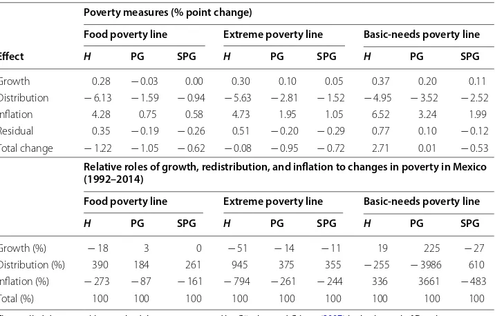
Table 1 shows the results corresponding to the period 1992–2014. The decomposition results are presented in the upper part of the table, while the relative impacts of growth, redistribution, and inflation on poverty, estimated from the decomposition results without considering the residual, are shown at the bottom. According to the results, the reduction of poverty at all levels was primarily explained by the important effect of redistribution, which accounted for the lion’s share of the decline in the long run. Growth only contributed marginally to the decline of food poverty as represented by the poverty gap (PG), whereas it was poverty-augmenting when considering the headcount index (H) of food poverty or any other indicator related to extreme and basic-needs pov-erty. This means that income growth was totally insufficient to raise the incomes of the poor and some non-poor as well in real terms during 1992–2014 to allow them to satisfy their basic needs, and therefore counteracted the beneficial impact of the lower levels of inequality that were observed (see Fig. 3).
Another important finding relates to the large impact of inflation on augmenting pov-erty. Regardless of the poverty line and measure that is used, the higher levels of inflation
facing the poor, as explained in the previous section (see Fig. 2), eroded most of the gains of a more equal society. In fact, when analyzing the higher poverty line of basic needs, inflation completely nullified the poverty-reducing impact of redistribution and, together with the negative income growth that is observed during the period (see Fig. 1), effectively increased the poverty level in the 22-year period of analysis.
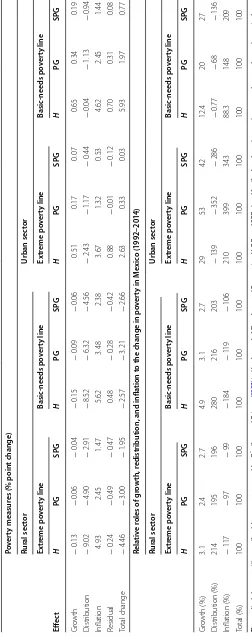
Table 2 shows the decomposition results by rural and urban sectors. We find stark dif-ferences between them, indicating that there are heterogeneous impacts of growth and inequality on poverty that are prevalent in each sector. It should be noted, first, that extreme and basic-needs poverty declined 4.46 and 2.57 percentage points, respectively, in the rural sector, whereas it increased 2.63 and 5.93 percentage points, respectively, in the urban sector during the period of analysis. It is evident from the results in the lower part of the table that the poverty decline in the rural areas is mainly owed to the strong poverty-reducing impact of redistribution, combined with a positive, albeit small, effect of income growth. These latter impacts strongly counteracted the persistently negative effect of inflation on poverty, contributing clearly to its decline regardless of the poverty measure that is used.
On the other hand, the situation in the urban sector was quite different because of three main reasons. First, growth was no longer poverty-reducing, but poverty-aug-menting during 1992–2014, which indicates that the growth of real income in the urban areas is actually lagging behind and became insufficient to provide a higher or even con-stant purchasing power of basic needs to the urban poor and some non-poor over time. Second, while the impact of redistribution was still positive as in the rural sector, its magnitude was smaller, particularly when evaluating its effect on basic-needs poverty. Third, according to the decomposition results, the phenomenon of higher prices facing
Table 1 Decomposition of changes in national poverty in Mexico into its growth, distribution, and inflation components (1992–2014)
The applied decomposition methodology was proposed by Günther and Grimm (2007) in the Journal of Development Economics. H, PG, and SPG stand for the headcount, poverty gap, and squared poverty gap indexes, which are part of the FGT poverty measures
Poverty measures (% point change)
Food poverty line Extreme poverty line Basic-needs poverty line
Effect H PG SPG H PG SPG H PG SPG
Growth 0.28 − 0.03 0.00 0.30 0.10 0.05 0.37 0.20 0.11
Distribution − 6.13 − 1.59 − 0.94 − 5.63 − 2.81 − 1.52 − 4.95 − 3.52 − 2.52
Inflation 4.28 0.75 0.58 4.73 1.95 1.05 6.52 3.24 1.99
Residual 0.35 − 0.19 − 0.26 0.51 − 0.20 − 0.29 0.77 0.10 − 0.12 Total change − 1.22 − 1.05 − 0.62 − 0.08 − 0.95 − 0.72 2.71 0.01 − 0.53 Relative roles of growth, redistribution, and inflation to changes in poverty in Mexico (1992–2014)
Food poverty line Extreme poverty line Basic-needs poverty line
H PG SPG H PG SPG H PG SPG
Growth (%) − 18 3 0 − 51 − 14 − 11 19 225 − 27
Distribution (%) 390 184 261 945 375 355 − 255 − 3986 610 Inflation (%) − 273 − 87 − 161 − 794 − 261 − 244 336 3661 − 483
Table
2
Dec
omp
osition of changes in r
ur al and ur ban p ov er ty in M exic o in to its gr
owth, distribution, and infla
tion c
omp
onen
ts (1992–2014)
The applied dec
omposition methodology w
as pr
oposed b
y Gün
ther and Gr
imm (
2007
) in the Jour
nal of D
ev
elopmen
t E
conomics
. H, PG, and SPG stand f
or the headc
oun
t, po
ver
ty gap
, and squar
ed po
ver
ty gap inde
xes
,
which ar
e par
t of the FGT po
ver ty measur es Po ver ty measur
es (% poin
the poor in Mexico seems to affect more severely the have-nots in the urban than in the rural areas.
It is therefore clear from the results in Tables 1, 2 that redistribution has played an important, unique role in the fight against poverty in Mexico during the last dec-ades. Without the income equalization process that has slowly taken place since 1998 (Iniguez-Montiel 2011; Cortés 2013; Lustig et al. 2013) in both the urban and rural sec-tors, with the implementation of programs such as Oportunidades and the Popular Health Insurance, food and extreme poverty would be much higher today than they were in the early 1990s, due to the income stagnation characterizing the Mexican economy since the 1980s debt crisis, as well as the soaring food prices affecting strongly the poor in Mexico since 2008 (CONEVAL 2013, 2015).
3.2.2 1992–2010
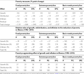
As the growth rate was lower in 1992–2010 than in 1992–2014, mainly because of the 2008–2009 economic recession led by the USA financial crisis, the contribution of improved income distribution to poverty reduction in Mexico becomes much more evi-dent in the former than in the latter period, whereas reduced income levels had a clear adverse impact on poverty by the end of the last decade as expected. These patterns hold regardless of the poverty line and measure used.
As shown in Table 3, both the decline of income growth as well as the increase in the real value of the poverty line contributed invariably to the partial increase of poverty, whereas lower income inequality in Mexico effectively countered the poverty-augment-ing impact of lower levels of income and heterogeneous inflation, reducpoverty-augment-ing the level of poverty consistently during the period. It should be noted that the negative effect of growth on poverty is not minor, accounting for approximately 23–38% of the partial rise in the headcount measure, whereas the remaining 62–77% was due to the higher prices of food in 2010, compared to 1992 (see Table 3, lower panel).6
We may therefore conclude that redistribution (lower income inequality) has played a crucial role in alleviating poverty in Mexico at all levels between 1992 and 2014, whereas unstable, slow growth as the one characterizing the Mexican economy has had little positive or even negative impact on reducing permanent (structural) poverty as shown in Tables 1, 2 and 3.7 How individual policies such as Oportunidades and the Popular
Health Insurance programs contributed to the improvement in income distribution is beyond the scope of this study. Instead, we attempt to elucidate the dynamic relationship between growth, inequality, and poverty from a different angle, using parametric regres-sions. This is the theme of the next section.
7 According to Hernández-Laos and Benítez-Lino (2014), household mobility to enter or exit permanent poverty is con-ditioned by the long-run growth of the economy. In contrast, in the short and medium run, the mobility possibilities of households are determined by the phases of the economic cycle, specially by changes in unemployment.
4 Panel analysis of regional data
4.1 Theoretical discussion
Three main hypotheses are tested for the case of Mexico in this paper. We discuss them briefly in this section to emphasize theoretical mechanisms underlying the sys-tem of equations to be presented and estimated in the following sub-sections. First, the hypothesis of the impact of inequality on economic growth has been long dis-cussed in economics, supported by two, contrasting ideologies. On the one hand, the view that inequality should be growth-enhancing is based on three arguments (Aghion et al. 1999): the rich’s higher tendency to save, investment indivisibilities, and a trade-off between efficiency and equity. On the other hand, according to the new growth theories, inequality is harmful for growth (Aghion et al. 1999; Alesina and Rodrik 1994; Perotti 1992, 1993, 1996; Persson and Tabellini 1994; Stiglitz 2012; among others). The harm may occur through political instability (Alesina and Per-roti 1996), high levels of criminality (Fajnzylber et al. 2002; Enamorado et al. 2016), or credit-market imperfections when agents are heterogeneous (Aghion et al. 1997;
1999).
The second hypothesis to be tested in this study proposes a reverse causality run-ning from growth to inequality. The most influential view related to this relationship
Table 3 Decomposition of changes in national poverty in Mexico into its growth, distribution, and inflation components (1992–2010)
The applied decomposition methodology was proposed by Günther and Grimm (2007) in the Journal of Development Economics. H, PG, and SPG stand for the headcount, poverty gap, and squared poverty gap indexes, which are part of the FGT poverty measures
Poverty measures (% point change)
Food poverty line Extreme poverty line Basic-needs poverty line
Effect H PG SPG H PG SPG H PG SPG
Growth 0.6 0.2 0.1 0.5 0.2 0.1 4.1 0.01 0.2
Distribution − 4.2 − 1.4 − 0.6 − 4.2 − 1.9 − 0.9 − 13.3 − 2.0 − 1.7
Inflation 1.6 0.6 0.3 1.5 0.8 0.4 6.9 0.7 0.7
Residual − 0.2 − 0.2 − 0.1 − 0.1 − 0.2 − 0.1 0.5 − 0.1 − 0.1 Total change − 2.20 − 0.84 − 0.40 − 2.3 − 1.07 − 0.57 − 1.76 − 1.42 − 1.00
Relative roles of growth, redistribution, and inflation to the reduction of poverty in Mexico (1992–2010)
Food poverty line Extreme poverty line Basic-needs poverty line
H PG SPG H PG SPG H PG SP
Growth (%) − 29 − 27 − 19 − 21 − 27 − 25 − 183 − 1 − 20
Distribution (%) 207 214 206 190 210 214 586 149 195
Inflation (%) − 78 − 87 − 87 − 69 − 83 − 89 − 303 − 48 − 75
Total (%) 100 100 100 100 100 100 100 100 100
Poverty-augmenting effect of growth and inflation in Mexico (1992–2010) Food poverty line Extreme poverty line Basic-needs poverty line
H PG SPG H PG SPG H PG SPG
Growth (%) 27 23 18 23 24 22 38 2 21
Distribution (%) 73 77 82 77 76 78 62 98 79
is the so-called Kuznets hypothesis. However, following a worldwide pattern of rising inequality since the 1980s (Atkinson 1997, 1999, 2004; Addison and Cornia 2001), it is now widely agreed that the distribution of income is not only determined by eco-nomic forces, but also by various political and social factors (Aghion et al. 1999), and therefore it is basically impossible to generalize about the evolution of inequality for all countries as Kuznets hypothesized. In this respect, several hypotheses have been proposed related to the determinants responsible for shaping the income or wealth distribution in each country. In the case of Mexico, for instance, the income distri-bution literature has primarily focused on the study of wage inequality in order to explain the observed increases in the skill premium (SP),8 which apparently occurred
right after the insertion of the economy into the global market and until 1996.9 In
particular, there are three competing hypotheses about the documented rise in wage inequality in Mexico during the 1980s and mid-1990s (Cortez 2001): an increase in the demand for skilled labor; changes in the distribution of education; and changes in labor-market institutions, namely, minimum wages and unionization rates.
Finally, two additional hypotheses, related to the impact of growth and inequality upon poverty, are also validated in this paper. Economic growth and the level of inequality are considered as the two main determinants of the poverty level.10 Whereas growth is said
to have a negative impact on poverty, the opposite effect holds true in the case of the dis-tribution of income. Therefore, on the one hand, economic growth reduces poverty, and an economic downturn increases it generally. On the other hand, an improvement along the distribution of income reduces poverty, while an inequality rise increases the poverty level correspondingly (Iniguez-Montiel 2014).11 The empirical literature on this issue
validates both hypotheses (Bourguignon 2004; Datt and Ravallion 1992; Iniguez-Montiel
2014; Kurita and Kurosaki 2011; Lopez 2006; Ravallion 1997, 2001, 2005; Ravallion and Chen 2003), and has also shown that higher initial inequality tends to reduce the posi-tive, decreasing impact of growth upon absolute poverty (Lopez 2006; Lopez and Ser-ven 2006; Ravallion 1997, 2005; Campos-Vázquez and Monroy 2016), through its direct, growth-inhibiting effect discussed above.
4.2 Empirical model
Following the standard in the literature and based on the economic theories discussed above, we estimate a system of equations that characterize dynamic changes that
8 The skill premium (SP) may be defined as the wage gap between low- and high-skilled workers or the ratio of white-collar workers to blue-white-collar workers.
9 The SP grew steadily during the 1980s and 1990s in Mexico, which implemented a large trade reform in the mid-1980s and was continually exposed to other forms of globalization, such as outsourcing or foreign direct investment, for the next two decades (Goldberg and Pavcnik 2007).
10 As discussed in Bourguignon (2004), Dagdeviren et al. (2004), and Lopez (2006), poverty is determined invariably by income growth and its distribution.
occurred between growth, inequality, and poverty. More concretely, denoting each state by subscript j, we estimate the following system of equations:
where Xjt is defined as a vector of observable factors, α stands for the unobservable and
time-invariant characteristics of state j, η represents unobservable macro shocks that affect all states in Mexico in period t, and ε is an idiosyncratic error term. The inclusion of α and η is also meant to minimize bias due to measurement errors associated with the non-representativeness of the original microdata at the state level (we also conduct other robustness checks to deal with the potential bias due to the non-representative-ness). Additionally, we estimate a model where income and inequality at time t deter-mine the current level of poverty for each state j as follows:
It should be noted that Eq. (3) is a revision of Eq. (4), which is the standard in the lit-erature, but which, as pointed out in Kurita and Kurosaki (2011), is likely to suffer from spurious correlation because the three variables of interest are dependent by construc-tion. By comparing the results from Eqs. (3) and (4), we can examine whether the bias due to such spurious correlation is serious.
Equations (1) and (2) can be estimated by a system generalized method of moments (GMM), a difference GMM, or a single-equation fixed-effect method, which is also used to estimate Eqs. (3) and (4). To estimate Eqs. (1), (2), (3) and (4), we used the state-level panel dataset that is balanced (384 observations = 32 states times 12 biannual observations from 1992 to 2014). The period t-1 thus implies 2 years before period t. When a single-equation fixed-effect method is applied to Eqs. (1), (2) and (3), the effec-tive sample size is 350, as we lose the first period observations due to the use of lagged dependent variables. When a difference GMM method is applied to Eqs. (1) and (2), the effective sample size is 320, as we further lose the second period observations due to the differencing for instruments. Finally, when a system GMM method is applied to Eqs. (1) and (2), the effective sample size becomes 350 again, because the additional condition
E
�yi,t−1εit
=0 that is added allows incorporating the levels and use yi,t−1 as an
instrument.
4.3 Empirical results
In this paper, we report estimation results based on the difference GMM estimation methodology proposed by Arellano and Bond (1991). The reason we report the differ-ence GMM results is that, according to the Arellano–Bond test, Eq. (2) is incorrectly specified when the system GMM methodology is applied to estimate the model and per-capita income is used as an independent variable, instead of per-per-capita consumption. Additional file 1: Appendix Table S1 reports the system GMM results for Eqs. (1) and (2). The first two columns correspond to per-capita consumption equations, whereas the
(1) lnyjt=β11lnyj,t−1+β12Ineqj,t−1+Xj,t−1θ1+α1j+η1t+ε1jt,
(2)
Ineqjt=β21lnyj,t−1+β22Ineqj,t−1+Xj,t−1θ2+α2j+η2t+ε2jt,
(3)
Povjt=β31lnyj,t−1+β32Ineqj,t−1+Xj,t−1θ3+α3j+η3t+ε3jt,
(4)
last two columns correspond to per-capita income equations. As it is possible to see in column 4 in both model specifications, the null hypothesis of no serial correlation in the residuals is rejected at the 5% level (Arellano–Bond test (Order 2)), which violates an important assumption indicating that the model is not correctly specified. Based on this important result, we decide not to use the system GMM estimates and to adopt the dif-ference GMM results to describe dynamic changes in the Mexican economy.12
4.3.1 Difference GMM results
Regarding yjt in the empirical model, we report results based on the mean consumption;
regarding Ineqjt, we report results based on the Gini coefficient; and regarding Povjt, we
report results based on the poverty headcount index. In calculating poverty measures for the empirical model, we used the official poverty lines corresponding to the extreme poverty. The robustness of our results with respect to these choices is discussed in sub-section 4.3 (c).
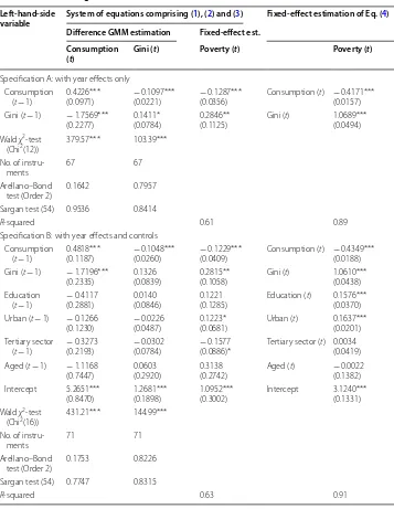
The estimation results of Eqs. (1), (2), (3) and (4) are shown in Table 4, first for a model with fewer controls and then for a model with more controls. Both models include state-specific effects ( αj ), but they are different in their lists of additional variables: one with year-fixed effects ( ηt ) only, and the other with ηt and Xj,t−1 (Education, Urban, Services,
and Aged).
All the coefficients of interest yield expected signs and are statistically significant. The income-convergence parameter ( β11) is estimated to be 0.42 and 0.48, both significantly
different from zero and one at the 1% level. This indicates that rapid income convergence exists within Mexican states and, therefore, that growth in Mexico is higher for those states whose initial consumption levels are lower, and vice versa, which is consistent with the conditional convergence hypothesis (Jones 2002).13
Similarly, the inequality-convergence parameter ( β22) is estimated to be between zero and one, and it is significantly different from zero at the 10% level in both models, and significantly different from one at the 1% level in both cases. This implies that inequality tends to decline faster in states with higher initial inequality, which is analogous to the inequality convergence found in Ravallion (2003).
The impact of inequality on subsequent growth, captured by the parameter coeffi-cient ( β12) , is estimated to be negative, as expected, and statistically significant at the 1% level. According to our estimations, the parameter is − 1.76 and − 1.72 in the model
with fewer and more control variables, respectively. This implies that an increase in the level of inequality, equivalent to one standard deviation (0.0449) in the Gini coefficient, reduces the level of growth in the next period by 0.0790 or 0.0772, or approximately 1.0% of the mean of Consumption. This is an economically significant number that suggests
12 By comparing the difference GMM results (Table 4) with the system GMM results (Additional file 1: Appendix Table S1, first two columns corresponding to per-capita consumption equations), it is possible to see that they are quan-titatively and qualitatively similar except for the inequality-convergence parameter ( β22) , which is not statistically
signifi-cant in the latter case in both model specifications. According to the Arellano–Bond- and Sargan-test results shown in the tables, the results of both estimators (difference GMM and system GMM) are all consistent because the errors are not serially correlated and the population moment conditions are correct as well.
that higher levels of inequality in Mexico have a negative impact on growth (which is one of the main theses suggested in Ros 2015), whereas lower levels of inequality tend to spur growth in the economy, as suggested by the new growth theories (Aghion et al.
1999; Alesina and Rodrik 1994; Benabou 1996).
The effect of growth on subsequent inequality, represented by parameter β21 , is nega-tive and statistically significant at the 1% level. These results imply that states in which initial levels of growth are higher tend to experience lower levels of inequality than states with lower levels of growth in the next period. They also suggest that growth contributes
Table 4 Difference generalized method of moments (GMM) estimation results
The number of observations is 320 for the difference GMM estimation, 352 for Eq. (3) and 384 for Eq. (4) Robust standard errors, adjusted for clustering on state, are shown in parentheses
***, **, and * represent significance at the 1, 5, and 10% level, respectively
Left-hand-side
variable System of equations comprising (1), (2) and (3) Fixed-effect estimation of Eq. (4) Difference GMM estimation Fixed-effect est.
Consumption
(t) Gini (t) Poverty (t) Poverty (t)
Specification A: with year effects only Consumption
(t − 1) 0.4226***(0.0971) −(0.0221) 0.1097*** −(0.0356) 0.1287*** Consumption (
t) − 0.4171*** (0.0157) Gini (t − 1) − 1.7569***
(0.2277) 0.1411*(0.0784) 0.2846**(0.1125) Gini (t) 1.0689***(0.0494) Wald χ2‑test
(Chi2(12)) 379.57*** 103.39*** No. of instru‑
ments 67 67
Arellano–Bond
test (Order 2) 0.1642 0.7957 Sargan test (54) 0.9536 0.8414
R‑squared 0.61 0.89
Specification B: with year effects and controls Consumption
(t − 1) 0.4818***(0.1187) −(0.0260) 0.1048*** (0.0409)− 0.1229*** Consumption (t) −(0.0188) 0.4349*** Gini (t − 1) − 1.7196***
(0.2335) 0.1326(0.0839) 0.2815**(0.1058) Gini (t) 1.0610***(0.0438) Education
(t− 1) −(0.2881) 0.4117 0.0140(0.0846) 0.1221(0.1285) Education (
t) 0.1576*** (0.0370) Urban (t− 1) − 0.1266
(0.1230) −(0.0487) 0.0226 0.1223*(0.0681) Urban (t) 0.1637***(0.0201) Tertiary sector
(t − 1) −(0.2193) 0.3273 (0.0784)− 0.0302 −(0.0886)* 0.1577 Tertiary sector (t) 0.0034(0.0419) Aged (t − 1) − 1.1168
(0.7447) 0.0603(0.2920) 0.3138(0.2742) Aged (
t) − 0.0022 (0.1382) Intercept 5.2651***
(0.8470) 1.2681***(0.1898) 1.0952***(0.3002) Intercept 3.1240***(0.1331) Wald χ2‑test
(Chi2(16)) 431.21*** 144.99*** No. of instru‑
ments 71 71
Arellano–Bond
test (Order 2) 0.1753 0.8226 Sargan test (54) 0.7747 0.8315
to reducing inequality in Mexico, as suggested in Ros (2015), in a similar fashion as the one Kuznets (1955) predicted for countries with a comparable level of development as Mexico.
The estimated parameters for Eq. (3) yield the expected signs and are statistically sig-nificant at the 1 or 5% level. In both versions of the model, the results imply that growth and inequality have a negative and positive impact on poverty, respectively. It should be noted that the parameter coefficient for inequality ( β32 : 0.2846 and 0.2815) is much
larger in absolute value than the growth parameter ( β31 : − 0.1287 and − 0.1229) in both versions of the model, which suggests that a change in the inequality level has a stronger poverty-reducing effect than that of growth.14
4.3.2 Bias due to spurious correlation
The results of Eq. (4) are also shown in Table 4. Again, the coefficients have the expected signs and are statistically significant at the 1% level, reinforcing the results and our inter-pretation of the parameters obtained for Eq. (3). However, as explained in Kurita and Kurosaki (2011), the coefficients in Eq. (4) are more susceptible to spurious correlation than those in Eq. (3) because the three variables of interest (consumption, inequality, and poverty) are calculated from the same microdata for the same year. Consequently, as far as the dynamic effects of growth and inequality on poverty are concerned, the esti-mated parameters in Eq. (3) in Table 4 are better indicators than those in Eq. (4).
Comparing the key parameters, the poverty-reducing impact of improved distribu-tion ( β32 ) is approximately 0.28 when proper lag structure is used (Eq. (3)), whereas it is
approximately 1.06 when no lag is allowed (Eq. (4)); the poverty-reducing impact of eco-nomic growth ( β31 ) is approximately − 0.12 when proper lag structure is used (Eq. (3)), whereas it is approximately − 0.43 when no lag is allowed (Eq. (4)). Therefore, the spuri-ous correlation overestimates the real dynamic relationship between poverty reduction and inequality reduction (or income growth) as suggested in Kurita and Kurosaki (2011).
4.3.3 Robustness checks
We ran a series of robustness checks of the results discussed so far and report the sum-mary results in Additional file 1: Appendix.
First, to investigate potential bias due to the non-representativeness of the state-level panel data, we attempt two different strategies. First, we restrict the sample used for the regression to a subsample comprising state-year observations in which at least 50 households were interviewed in the urban sector only. The results are shown in Addi-tional file 1: Appendix Table S2, which are quantitatively and qualitatively similar to those in Table 4. A notable change is that the absolute value of the inequality-conver-gence parameter ( β22 ) becomes larger under the model with controls and now statisti-cally significant. This confirms our interpretation of the main result that the parameter is
14 To see this more clearly, according to our estimates, when inequality decreases by 1%, poverty decreases by 0.28%. On the other hand, when income/consumption increases by 1%, poverty decreases by 0.0013%. These two parameters ( β31 and β32 ) are not immediately comparable because income/consumption is expressed in logarithmic form, whereas
between 0 and 1. Second, following Hernández-Laos and Benítez-Lino (2014), we com-pile an alternative panel dataset from 2005 to 2014 by using the Mexican labor force survey (quarterly data),15 which is representative at the state level. One drawback of
this approach is that the labor force survey reports only labor income. However, as the labor income accounts for about 66% of total current income and 80% of total monetary income in Mexico (Hernández-Laos and Benítez-Lino 2014), the drawback is not likely to be serious enough to make the robustness check ineffective. The results in Additional file 1: Appendix Tables S3, S4 have the same signs with similar or higher statistical sig-nificance levels as those reported in Table 4. From these robustness-check results, we conclude that our main results are not affected by the bias due to the non-representa-tiveness of the data at the state level.
Second, it is well known that Arellano–Bond GMM results may be sensible to the instruments and lags included in the estimation. As we have already discussed above regarding the choice between system and difference GMM, we re-estimate the main model using longer lags. The estimation results are reported in Additional file 1: Appen-dix Table S5. All of the additional lags have insignificant coefficients and our main parameters of interest ( β11 , β12 , β21 , and β22 ) remain similar to those reported in Table 4.
Third, as the period 2008–2010 experienced the negative effects of a severe recession after the USA financial crisis (see Sect. 2), which affected the Mexican economy differ-ently than the rest of Latin America as well as other developing and emerging markets (Hernández-Laos and Benítez-Lino 2014), we examine the robustness of our results by restricting the period of analysis to 2010 (excluding 2012 and 2014), and we found that all the results are quantitatively and qualitatively similar to those for the period 1992– 2014 (see Additional file 1: Appendix Table S6).
Fourth, as shown in Sects. 2 and 3, the official poverty lines in Mexico were not con-stant over time in real terms if adjusted according to the national CPI. To control for this problem, we re-calculated the poverty measures using our own poverty lines, which are constant over time, and re-estimated the equations (see Additional file 1: Appendix Table S7). Again, all of the results turned out to be quantitatively and qualitatively simi-lar to the default results discussed above.
Fifth, regarding yjt in the empirical model, we re-estimated the model by replacing
mean consumption per capita by mean income per capita in each state in real pesos. Since the results are qualitatively similar (see Additional file 1: Appendix Table S8), we continue our discussion using the mean consumption but interpret it as the proxy for the mean income as well.
Sixth, regarding Ineqjt in the empirical model, we re-estimated the model by
replac-ing the Gini coefficient by two different inequality measures. The first one is the mean income ratio of the top quintile (80th percentile) to the bottom quintile (20th percentile) and the second one is the mean income ratio of the top decile (90th percentile) to the median. The motivation of using the 80/20 ratio is a simple robustness check. Similar to the Gini index, the 80/20 ratio takes into consideration the distributional change that
occurs to the poor. Unlike the Gini index, the 80/20 ratio gives less weight to the seg-ments of the population in the middle. The results using the 80/20 ratio are qualitatively similar (see Additional file 1: Appendix Table S9), but there are some important differ-ences as expected. First, the impact of inequality on subsequent growth (parameter β12 ) has the expected sign but is smaller in magnitude, which may imply that the reduction of inequality between the very poor and the very rich is less important to economic growth than when inequality among all members of society is considered as the new growth theories predict. Second, the effect of growth on subsequent inequality (parameter β21 ) has the expected sign but is considerably smaller in magnitude, implying that growth has weak effect on the inequality between the poorest and richest segments of the popula-tion. Finally, the income and inequality elasticities of poverty (parameters β31 and β32 ) have the expected signs in both models, but, in contrast with the main results, the ine-quality elasticity is much smaller in absolute value than the growth elasticity.
The motivation of using the 90/50 ratio is different. Unlike the Gini index or the 80/20 ratio, changes in the 90/50 ratio do not directly affect the poor, as the poverty headcount index in Mexico is mostly below 50%. Therefore, by using the 90/50 ratio, we can clearly identify the indirect effects of inequality on poverty and economic growth, such as those working through the rich’s incentives to invest or political-economy mechanisms faced by the rich (see subsection 4.1). Additional file 1: Appendix Table S10 shows the estima-tion results when the 90/50 ratio is used as the inequality measure. Substantial differ-ences are found when focusing on the model with more controls. First, the 90/50 ratio has little or no impact on subsequent growth as implied by the statistical insignificance of parameter β12 . Likewise, parameter β21 is also not statistically significant in the speci-fication with controls, implying that the effect of subsequent growth on this inequal-ity index is null. Finally, the impact of inequalinequal-ity on subsequent poverty, represented by parameter β32 , is also non-existent given the statistical insignificance of the parameter
coefficient. Therefore, it is possible to conclude from the results of this test that distri-butional changes that occur in the lower half of the population distribution matter for poverty reduction and economic growth. In other words, the 90/50 inequality ratio is not dynamically related to growth and poverty in Mexico probably because the rich’s economic status is isolated from the economic status of the mass, including the poor. This possibility is worth further investigation, left for future research.
4.4 Re-interpreting the decomposition results regarding the impact of improvement in distribution on poverty reduction
A closer look at Fig. 3 suggests a discontinuity around 2002. If we use national fig-ures, the Gini coefficients were stable at approximately 54% until 2000, whereas they fell to a level of approximately 52% for the period 2002–2008. Therefore, we run a back-of-the-envelope calculation16 of impacts of a one-time shock to Eq. (2) that reduces the
Gini coefficient by 2 percentage points (or a 4% decline in the inequality level without the shock) in year 2002 in all states in Mexico. In the next period (2004), the poverty headcount index would decline by approximately 1.13% (0.2815 times − 4). In the same year, the average consumption would increase by approximately 6.88% (− 1.7196 times − 4), whereas the Gini coefficient would decrease by approximately 0.53% (0.1326 times
− 4). After one more interval (2006), the poverty headcount index would decline further by approximately 0.99%, through both the reduction of income inequality (0.2815 times
− 0.53) and the increase in average consumption (− 0.1229 times 6.88) in 2004.
The persistence of the shock, however, dies away with time, because our parameter estimates predict a system convergence. The accumulated impact until 2014 can be cal-culated by multiplying six times the 3 × 3 matrix of parameters with (0.4818, − 1.7196, 0) in the first row, (− 0.1048, 0.1326, 0) in the second row, and (− 0.1229, 0.2815, 0) in the third row. The third row of the matrix after multiplication becomes (− 0.0309, 0.0838,
0). Therefore, the persistent impact on poverty in 2014 of the shock in income distribu-tion in 2002 would be a decline in the headcount index by approximately 0.34% (0.0838 times − 4). Although much smaller than the immediate impact, the persistent effect after 12 years is still substantial.
The simple calculation in this subsection thus explains why the inequality reduc-tion during the period 1992–2014 was mainly responsible for the reducreduc-tion in poverty in Mexico, as we demonstrated in our decomposition in Sect. 3. Another observation in Sect. 3 (i.e., for the period 1992–2010), which is that changes in the level of growth counteracted the positive effect of inequality on poverty, partially increasing the poverty level, could be understood in a similar way as an unexpected negative shock to average consumption in 2010.
5 Conclusions
Using micro datasets of households collected during the period 1992–2014, we exam-ined the contributions of growth and redistribution to poverty reduction in Mexico. In the first part of our analysis, we used household-level data as repeated cross sections and decomposed the observed changes in poverty reduction in Mexico into components arising from growth, improved distribution, and heterogeneous inflation. We found the component of inflation to be non-negligible and highly detrimental to the poor in both the rural and urban areas, which is only the natural result of the higher and increas-ing prices of food experienced by the poor since 2008. The decomposition also shows improvement in income distribution to be the main contributor to poverty reduction in Mexico during the period 1992–2014 and the only factor that was responsible for the decline in poverty during 1992–2010, a period characterized by economic instability
(Hernández-Laos and Benítez-Lino 2014; Iniguez-Montiel 2014), low growth rates (Ros
2015), and where the benefits from growth accruing to the poor literally disappeared due to the severe economic recessions affecting the country in 1994–1995 and 2008– 2009. However, 2010 was the year with the lowest level of inequality recorded in Mexico since the late 1980s, which was similar to the level of inequality in 1984 (Cortés 2013). According to a rough estimation, redistribution alleviated poverty in Mexico from 1992 to 2010 by increasing the incomes of the poor by 9% and 5% in the rural and urban sec-tors, respectively.
In the second part of our analysis, we compiled a unique panel dataset at the state level and characterized the dynamic relationship between growth, inequality, and poverty, being careful to avoid spurious correlation arising from data construction. The GMM regression results show that Mexican states are characterized by income convergence and inequality convergence, that lower levels of inequality spur growth in the economy, that increasing income/consumption levels contribute to reducing inequality, and that poverty reduction in Mexican states is highly determined by inequality (rather than income) levels in the previous period. Indeed, the growth and inequality elasticities of poverty found in our results provide evidence of the stronger poverty-reducing impact of redistribution for middle-income, high-inequality countries as suggested in the litera-ture (Dagdeviren et al. 2004; Lopez 2006). As we also found that inequality has a harmful effect on growth, consistent with the findings and conclusions in other studies (Aghion et al. 1999; Cingano 2014; Ros 2015; Stiglitz 2012), once a small perturbation occurs in a state that reduces the inequality level, the state is expected to experience sustained income growth and accelerated poverty reduction simultaneously. The back-of-the-envelope calculation of the dynamic response of poverty to a shock (reduction in income inequality) indeed shows that the impact is persistent.
We, therefore, conclude that growth becomes more inclusive and stable in Mexico if the country adopts an active, pro-poor growth policy (Iniguez-Montiel 2014) that can further reduce inequality. In addition, given the low growth of the Mexican economy since the 1980s as well as the asymmetrical and heterogeneous impact of that growth on poverty within each state during economic expansions and recessions (Campos-Vázquez and Monroy 2016), it appears that a different development strategy such as the one out-lined in Ros (2015)—one that can truly spur the economic growth of the country, par-ticularly that of the rural sector (McKinley and Alarcon 1995) and the south of Mexico, by increasing public investment/infrastructure, expanding the domestic market (rather than relying primarily on export-led growth and the growth of the USA economy), while reducing inequality as well as poverty at a faster pace—should be adopted.
as a whole during economic contractions, which nullify the rather small advances made during growth spells (Campos-Vázquez and Monroy 2016). Therefore, equity should play a key role in Mexico’s development process (Iniguez-Montiel 2011, 2014; Ros 2015; Torres and Rojas 2015) by creating and promoting the necessary institutions that would allow all citizens to expand their economic opportunities and political rights (Acemo-glu and Robinson 2013). It should be specially so given the negative, reverse causalities (between growth and inequality) identified in this study, which could be at the heart of the main vicious cycles in the economy. If these important dynamic relationships con-tinue to be ignored by policymakers and economic elites, the consequences for Mexico could be even more disastrous than the great imbalances, costs, and bad outcomes that have been delivered over the last decades (Acemoglu and Robinson 2013; Cingano 2014; Enamorado et al. 2016; Iniguez-Montiel 2011; Ros 2015; Torres and Rojas 2015).
Additional file
Additional file 1. Appendix.
Authors’ contributions
AJIM gathered the data, compiled the panel datasets, carried out the analyses, created tables and figures, interpreted the results and drafted/revised the manuscript. TK interpreted the results, carried out the back‑of‑the‑envelop calculation, re‑interpreted the decomposition results in Sect. 4.4 and revised the manuscript. Both authors read and approved the final manuscript.
Author details
1 Graduate School of Economics, The University of Tokyo, 7‑3‑1 Hongo, Bunkyo, Tokyo 113‑0033, Japan. 2 Institute of Eco‑
nomic Research, Hitotsubashi University, 2‑1 Naka, Kunitachi, Tokyo 186‑8603, Japan.
Acknowledgements
The authors are grateful to the anonymous reviewer of this journal, Carlos A. Ibarra Niño, Masamune Iwasawa, Daiji Kawa‑ guchi, Yoko Kijima, and Jaime Ros Bosch for very constructive comments and suggestions that contributed to improving our study considerably. Additionally, we wish to thank seminar participants at the Institute of Developing Economies (IDE‑JETRO), the 5th Congress on Economics and Public Policy “Sobre México” at Iberoamericana University, the Japanese Economic Association Meeting at Sophia University, the JICA Research Institute, and the University of Tsukuba for helpful comments and discussions. Iniguez‑Montiel acknowledges financial support from the Japan Society for the Promo‑ tion of Science (JSPS), as well as invaluable non‑financial support from Koichi Ushijima at the University of Tsukuba Any remaining errors are our own.
Competing interests
The authors declare that they have no competing interests.
Publisher’s Note
Springer Nature remains neutral with regard to jurisdictional claims in published maps and institutional affiliations.
Received: 3 October 2016 Accepted: 23 July 2018
References
Acemoglu D, Robinson J (2013) Why nations fail: the origins of power, prosperity and poverty. Crown Publishing Group, New York
Addison T, Cornia GA (2001) Income distribution policies for faster poverty reduction, UNU‑WIDER discussion paper 2001/93. UNU‑WIDER, Helsinki
Aghion P, Banerjee A, Piketty T (1997) Dualism and macroeconomic volatility, mimeo. University College, London Aghion P, Caroli E, Garcia‑Penalosa C (1999) Inequality and economic growth: the perspective of the new growth
theories. J Econ Lit 37(4):1615–1660
Alesina A, Perroti R (1996) Income distribution, political instability, and investment. Eur Econ Rev 40(6):1203–1228 Alesina A, Rodrik D (1994) Distributive politics and economic growth. Quart J Econ 109(2):465–490