Earth before life

R E S E A R C H

Open Access

Earth before life

Caren Marzban

, Raju Viswanathan

and Ulvi Yurtsever

Abstract

Background: A recent study argued, based on data on functional genome size of major phyla, that there is evidence life may have originated significantly prior to the formation of the Earth.

Results: Here a more refined regression analysis is performed in which 1) measurement error is systematically taken into account, and 2) interval estimates (e.g., confidence or prediction intervals) are produced. It is shown that such models for which the interval estimate for the time origin of the genome includes the age of the Earth are consistent with observed data.

Conclusions: The appearance of life after the formation of the Earth is consistent with the data set under examination. Reviewers: This article was reviewed by Yuri Wolf, Peter Gogarten, and Christoph Adami.

Keywords: Genome, Evolution, Origin, Regression, Measurement error, Confidence interval, Prediction interval

Background

Sharov [1], and more recently, Sharov and Gordon [2] reported an analysis of data on the evolution of genetic complexity during the history of life on Earth. These two works - hereafter denoted SG - use the functional genome size of major phylogenetic lineages, as a measure of genetic complexity, and show that it has an exponen-tial relationship with the estimated dates of the transitions where these lineages first originated. As such, there exists a linear relationship between the logarithm of genome size (y) and the transition date (x). SG performed regression on a data set onyvs.x, and proposed that thex-intercept of the fit (i.e., where genome size is zero) provides an estimate for the age of life.

The work was criticized on many levels, ranging from the manner in which the data was produced, to the way in which the data was analyzed. A fundamental prob-lem is the paucity of data over the first 2 billion years or so of Earth’s history, resulting in large uncertainties in functional genome size at specific times. For instance, for prokaryotes, the size of the functional genome is guessed from the smallest present-day prokaryote genome. Exactly when this genome size evolved is a matter of conjecture;

*Correspondence: [email protected]

1Applied Physics Laboratory, Univ. of Washington, Seattle, WA, 98105-6698, USA

2Department of Statistics, Univ. of Washington, Seattle, WA, 98195-4322, USA Full list of author information is available at the end of the article

although an approximate date can be estimated from molecular clock type evolution rates based on more recent organisms (see e.g., the reviews of [1]), rates of increase of functional genome size could have been very different in the distant past. Fitting the data with an extrapolation based on a single, fixed rate of increase could lead to possi-bly incorrect conclusions. Likewise, the use of only coding regions of the genome as a measure of genome complexity has been pointed out as a potential problem, as non-coding regions could play a regulatory role and the asso-ciated complexity is unaccounted for when only coding regions are measured. Thus estimating genome complex-ity of extinct organisms based on an uncertain estimate of functional genome size of present-day organisms could be doubly flawed.

In addition to all of the above criticisms, there are addi-tional concerns over the statistical analysis in SG. First, and foremost, is the way in which the regression fit is used to extrapolate far beyond the range ofxvalues appearing in the data. It is well known that extrapolation can lead to misleading conclusions [3]), and so, any conclusions regarding the age of life, based on extrapolation, should be considered with extreme caution. A second aspect of the SG regression fit is that it does not incorporate statis-tical uncertainty due to sampling variability, e.g., through confidence or prediction intervals. The inclusion of such intervals can lessen the misleading impacts of extrapo-lation, because they generally widen as one moves away

from the mean of the data [4]. When an interval esti-mate is produced for thex-intercept, then the age of life can be estimated to within a range of possible values. Val-ues outside of the interval may be rejected (with some confidence), but all of the values within the interval are possible, and in fact, equally “likely.” As such, consider-ation of interval estimates is important because it can mitigate misleading conclusions.

Another limitation of the SG regression analysis is that it does not systematically account for uncertainty in the dates at which the transitions occurred (i.e., the

x-values of the data), also known asmeasurement errors.

As explained here, measurement errors generally reduce the slope of the regression fit, and consequently increase the value of the x-intercept. As such, failure to account for measurement errors leads to overestimates for the age of life. Regression models which systematically take measurement errors into account are calledmeasurement error models[5,6].

In this paper, a simple measurement error model is developed for the SG data, and rudimentary interval esti-mates are produced for the fit. In such a framework, the age of life is estimated to be within a range of possible values, with the range itself depending on a quantity pro-portional to the variance of the measurement errors. In other words, an estimate of the age of life is contingent on an estimate of the typical error in the lineage transi-tion dates. An attempt is made to estimate the variance of the measurement errors, and it is shown that the pro-posed model is consistent with life having formed around 4.5-billion years ago. In short, we find that when the regression analysis involves interval estimates, and incor-porates measurement errors, then the data used by SG provide no evidence to support the claim that life must have formed prior to the formation of the Earth.

Method Regression effect

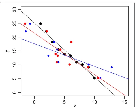
Consider a scatterplot ofyvs.x, displaying some amount of association between the two variables (e.g., Figure 1). It is well known that as the spread of the data increases, the slope of a least-squares fit approaches zero. This effect is known by a variety of names, includingthe regression effect

[7]. It is demonstrated in Figure 1, where the black, red, and blue circles are fictitious data with increasing error in

x; i.e, the black circles have less scatter than the red circles, etc. The straight lines are the ordinary least-squares fits to the respective data sets. It can be seen that increasing scatter leads to lower values of the slope.

The mathematics underlying the regression effect is straightforward. It is easy to show

ˆ

y(x)−y sy =

r(x−x sx

), (1)

Figure 1Demonstration of regression effect.The black, red, and blue circles show data sets with increasing errors inx-values. As a result, their ordinary least-squares fits have progressively smaller slopes.

where yˆ(x) is the predicted/fitted value,xand yare the sample mean ofxandy, respectively, andsx,sy are their

sample standard deviations. The quantity r is Pearson’s correlation coefficient, and measures the amount of scat-ter on the scatscat-terplot. Asrapproaches zero (from either side), the predicted valueyˆ(x)tends to the sample mean of y. Indeed, this “regression to the mean” is the reason why the least-squares fit is called regression [8]. In sum-mary, as the amount of scatter in the scatterplot ofyvs.

xincreases, the least-squares fit converges to a horizontal line with slope zero, and y-intercept equal toy.

Regression dilution

The aforementioned scatter may be due to errors inx, iny, or both. In the most common form of regression, the pre-dictorxis assumed to be error-free, and only the response

yis assumed to be subject to errors. Measurement error models [5,6] are designed to allow for bothxandyto be subject to errors. Consequently, as expected from the pre-vious example, measurement errors tend to “flatten” the least-squares line - a phenomenon calledregression dilu-tion [5,6]. Moreover, if the measurement errors can be estimated, then one can undo the dilution.

A simple measurement error model is as follows: Let

(Xi,Yi),i= 1,. . .,a, denote the true, error-free, values of

two continuous random variables satisfying the relation

Yi=α∗+β∗Xi. (2)

The corresponding observed values(xi,yi)can then be

written as

whereωi andi are the measurement error inXand the

error inY, respectively. For simplicity, it is assumed that both errors are normally distributed with zero mean, and variances given byσ_w2andσ2. I.e.,ωi∼N(0,σw2)andi∼ N(0,σ2). In thefunctional modeltheXis assumed fixed (non-random), but in thestructural model Xis assumed to be a random variable [5,6]. In other words, in the former, theavalues ofXiare assumed to be fixed quantities, while

in the latter they are considered to be a random sample taken from a population (or a distribution). The latter is adopted here because it is more appropriate for the prob-lem at hand, and for simplicity we assumeXi ∼N(μ,σ_b2).

The subscripts “b” and “w” are motivated by “between-group” and “within-“between-group” variances - language common to the analysis of variance formulation of regression [9].

If one mistakenly ignores measurement errors (inX), and instead performs regression on(xi,yi), i.e.,

yi=α+βxi+i, (4)

then it can be shown that the least-squares estimate of the regression slope and y-intercept are given by [5,6,10]:

β =β∗/λ , α=y−(β∗/λ)x , (5)

with

λ=1+σ 2

w

σ_b2 . (6)

Given that λ > 1, it follows that β < β∗, i.e., the slope is “diluted” relative to the slope that would have been obtained if measurement errors were zero. Therefore, as mentioned previously, measurement errors tend to flatten the least-squares fit, and thereby lead to an overestimate of the x-intercept. For the SG data, then, measurement errors lead to an overestimate for the age of life.

Equation (5) implies that one can correct this overes-timation by simply multiplying the observed regression coefficient β by λ[5,6,10]. In other words, the quantity (β λ) is an estimator ofβ∗. Similarly, the least-squares esti-mate ofα∗ is(y−(β λ)x). Note that in a measurement error model of the SG data, the estimate for the age of life is given by the correctedx-interceptx−y/(β λ). In order to make any of these corrections, however, one must estimateλ.

Frost and Thompson [11] discuss six methods for esti-matingλand the corresponding variance. One of the sim-pler methods examined there identifiesλ as the inverse of the intraclass correlation coefficient (also known as the reliability ratio). One advantage of that estimator is that its variance has a simple expression:

(λ2−1)2

a . (7)

In the following not only an attempt is made to estimate

λitself, we also consider the “inverse problem” of finding

the range ofλvalues which lead tox-intercepts consistent with 4.5 billion years as the age of life.

It is not necessary to find a specificλvalue which leads to anx-intercept of 4.5 billion years. A regression fit whose confidence or prediction interval includes anx-intercept of 4.5 billion years is sufficient, in the sense that it does not contradict the null hypothesis that life began after the for-mation of the Earth. In order to construct such an interval, one must compute the variance for the corrected regres-sion slope, a quantity which has been derived in [11]:

V[(β λ)]=λ2V[β]+1

a(β

2_+V[β])(λ2₋₁₎2_{. (8)}

where Equation (7) has been used.

There is an ambiguity in whether the appropriate inter-val for this problem is a confidence interinter-val or a prediction interval [4]. The former is designed to cover the true con-ditional mean ofy, givenx, a certain percentage of time, e.g., 95%. The latter is designed to cover a single predic-tion ofy, a certain percentage of time. By construction, the prediction interval is wider than the confidence inter-val. An argument in favor of using a prediction interval is that thex-intercept corresponds to a single prediction ofy. One can also argue that the appropriate interval is a con-fidence interval, because thex-intercept is technically a population parameter. The choice between the two inter-vals is of secondary importance. What is more important than the choice of the two intervals is thatsomeinterval must be considered. Here, a prediction interval is used; using confidence intervals leads to qualitatively similar conclusions.

The construction of prediction intervals in measure-ment error models is itself a complex issue and is consid-ered by [12]. One relatively simple 95% prediction interval is given byyˆ(x)±1.96σpe, whereσpe2 is the variance of the

prediction error, given by

σ_pe2 =σ2+σ 2

a +(X−X)

2_{V[βλ]+[(β λ)}2_{+V[β λ] ]σ}2

b ,

(9)

where V[(β λ)] is given by Equation (8), and σ2 is esti-mated by the variance of the residuals. This is the expres-sion derived in [12] for the special case where the value of X at which the prediction is made is a known (non-random) quantity. The first three terms on the right-hand side of Equation (9) are the variance of the prediction error in the error-free case [10]; the last term is the result of measurement errors.

Estimating measurement errors

One may wonder what is a typical value ofλfor the data at hand. Given Equation (6),σbandσwmust be estimated. To

ntimes. Denoting the resulting data asxij,i=1,. . .,a, j=

1,. . .,n, it is known that unbiased estimates ofσ_b2andσ_w2

are

(s 2

b n −

s2_w n) , s

2

w, (10)

respectively, withs2_bands2_wdefined as

s2_b= n a−1

a

i

(xi.−x..)2 , s2w=

1

a(n−1) a,n

i,j

(xij−xi.)2 .

(11)

where an overline denotes averaging over the index with a dot [9]. For largen, the quantitys2_b/nconverges to the sam-ple variance of theXi, i.e.,s2X = a−11

a

i(Xi−X)2, which

in turn can be estimated with the sample variance of the

xi. For the data at hands2_b/n ∼ 1.86 (billion years)2. In

the large-nlimit, the terms2_w/nconverges to zero, because in that limits2_witself converges to the constantσ_w2. There-fore, asymptotically,σ_b∼√1.86∼1.36 billion years.

The within-group standard deviation sw reflects the spread in values or uncertainty of the dates of appearance of the respective functional genomes (e.g., prokaryote, eukaryote, worms, fish, mammals). While the statistical analysis presented here assumes that theameasurements all have common variance (i.e., homoscedastic), in reality the uncertainty in the time of appearance of a functional genome increases from present to past. Thus the largest errors or uncertainties are found in the oldest functional genome considered. As an example of dating uncertainty, while the earliest mammals are believed to have arisen about 225 million years ago, based on early fossils [13], molecular clock studies based on genomes place mam-malian origins around 100 million years ago [14]. There is thus an uncertainty of the order of 100 million years or more in setting the time of the mammalian functional genome. The origin of eukaryotes has been identified to lie in the time interval between 2.3 billion and 1.8 billion years ago, thus with an uncertainty of 250 million years around the mean estimate of 2.05 billion years ago [15]. Early fossil evidence for prokaryotes in lava beds has been dated to a time around 3.5 billion years ago [16]; how-ever, it is unclear exactly when the functional genome size reached the present-day minimum value of around 5×105; the uncertainty in this time value could easily be of the order of 1 billion years.

Within-group standard deviations in the dates at which respective functional genome sizes were attained, there-fore, have an order of magnitude spread in range of val-ues, from 100 million to 1000 million years, with most standard deviation values being of the order of a few hun-dred million years. In a homoscedastic model of the type assumed in the present article, we will use as a rough (weighted) estimate a value ofsw∼500 million years.

Therefore, withσ_b ∼1.36 billion andσw ∼0.5 billion,

we haveλ ∼ 1.14 . For uncertainties around 100 million years,λis around 1.00, and it is around 1.54 if uncertainty is around 1 billion years.

Results and discussion

The formula for the prediction interval shown above depends on the quantityλ. In the previous subsection we arrived at a rough estimate for that quantity. Now, we examine the range ofλvalues which lead to conclusions consistent with the hypothesis that life did not begin prior to the formation of the Earth.

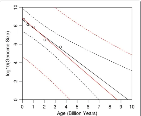
Figure 2 shows all of the results. The black line shows the ordinary least-squares fit to the data. It is the x -intercept of this line, i.e., about 9.5 billion years, which led SG to conclude that life must have begun prior to the formation of the Earth (i.e., about 4.5 billion years ago). The region between the black, dashed curves is the 95% prediction interval for the ordinary least-squares fit. According to this prediction interval (without taking mea-surement errors into account) life may have originated as early as 7 billion years ago.

The analogous results based on the above measurement error model are shown in red. The value ofλfor this fit is 1.14 - the value estimated in the previous section. Note that the resulting prediction interval includes 4.5 billion. In other words, ifλis about 1.14, then the results of the analysis do not reject the hypothesis that life began after

the formation of the Earth. Even aλas small as 1.1 leads to results (not shown here) consistent with 4.5 billion years as the age of life.

Although, a proper interpretation of prediction inter-vals correctly draws all focus away from the “center” of the interval, it is possible to arrange for the corrected fit itself to have anx-intercept of 4.5. The result is not shown here, but the corresponding value ofλis about 2.7. Values ofλin the 1.1 to 2.7 range are not uncommon; Frost and Thompson [11] even considerλvalues as large as 5. More importantly, that range includes theλvalues estimated in the previous section.

Based on Figure 2, note that the genome size at Age = 0 may be as low as 105(i.e., the lower limit of the predic-tion interval at Age = 0); one may be inclined to conclude that such a low value is unlikely. Also note that Age = 4.5 is only at the lowest limit of the possiblex-intercepts; one may then be inclined to conclude that Age = 8.5 (thex -intercept of the red line itself ) is the more likely estimate for the age of life. Although both premises are correct, the conclusions do not follow. The fallacy in both arguments is to attribute a likelihood to different regions within the prediction intervals. The correct interpretation of predic-tion (and confidence) intervals does not allow that type of interpretation [4]. Specifically, regarding Figure 2, all one can conclude is that about 95% of prediction intervals will cover genome size, at a given value of Age. More loosely stated, one can be “confident” that the true fit lies some-wherewithin the region between the red, dashed curves; nothing can be said about which of the possible fits (or their slopes and intercepts) are more, or less, likely.

The original conclusion of SG is a consequence of an incomplete analysis. Although the analysis presented here is more complete, many improvements are possible. For instance, nonlinear fits can made, and more refined mea-surement error models can be developed. The inference component of our analysis (i.e., the 1.96 appearing in the prediction interval formula) can also be improved upon. The assumption of homoscedasticity can be relaxed, the

σ_w and the σ_b can be estimated without the large-n

assumption, and one can even compute confidence and/or prediction intervals for thex-intercept itself. Lastly, data sets considerably larger than used by SG can be employed as genome size data is readily available for many major transitions along the tree of life (see, e.g., http://itol.embl. de/itol.cgi and http://www.ncbi.nlm.nih.gov/genome).

In short, many aspects of the above formulation are sim-plistic, approximate, or even controversial. As such, they offer avenues of further research. These limitations have not been of concern here because the main goal of the paper has been to introduce measurement error models and to highlight the importance of producing interval esti-mates of the fit. The details of the measurement error model, the manner in which the interval estimates are

generated, or whether the appropriate interval is a confi-dence or prediction interval, are all of secondary impor-tance because they affect the conclusions only in degree, not in kind.

Conclusions

A naïve regression model relating genome size to the age of life suggests that life may have formed prior to the Earth’s formation. Here we have shown that measurement errors lead to biased (i.e., over-) estimates for the age of life, and that the bias can be corrected/removed. Addition-ally, a more refined regression analysis is performed which 1) takes into account measurement errors, and 2) gener-ates interval estimgener-ates of the fit. The analysis depends on a parameter,λ, which is related to the variance of the mea-surement errors. We find that a wide range of plausible

λvalues lead to intervals that allow for life to have been formed more recently than 4.5 billion years ago, In short, the data analyzed by SG are consistent with the hypothesis that life may have formed after the Earth’s formation.

Reviewers’ comments

Reviewer’s report 1: Yuri Wolf, Institute of Cytology and Genetics, Novisibirsk, Russia

In a recent paper Sharov & Gordon (SG) infer the time-line of the growth of genomic complexity in the history of life and extrapolate the trend into the past. Strikingly, their analysis seems to contradict the origin of life on Earth since the x-intercept of the extrapolation indicates the age at least twice that of the Earth crust solidification. Here Marzban et al. offer criticism of this conclusion on the grounds of the SG failure to take into account the uncer-tainties in the estimates of the age of origin of major taxa. The authors give a brief but fair tally of multiple prob-lems with the SG analysis other than the focus of this work. I would like to emphasize that criticism on technical grounds by Marzban et al. does not imply that everything else is right about the SG approach. I consider this paper as an important and useful tutorial on regression using the problematic SG analysis as a teaching point, rather than an earnest attempt to show that the origin of Earth before life is compatible with the available data.

Two comments on the presentation

- The discussion of the relative likelihood of values within the prediction interval (p. 5 of the manuscript) is, in my opinion, either too superficial or superfluous. It would be interesting to see a full analysis of the relative likelihood of Age = 4.5 vs Age = 8.5 (preferably taking into account that errors in age estimates are not homoscedastic); other-wise it would be sufficient just to state that Age = 4.5 lies within the prediction interval and thus cannot be rejected.

A minor technical point

- The authors call the relationship of inferred genome complexity with the estimated dates of the origin of lin-eage “logarithmic” (p. 1 of the manuscript). Actually, a linear relationship between the logarithm of genome size and the transition date indicates exponential relationship between the genome size and the date (since the date is, unquestionably, the argument here).

Authors’ reply 1: We agree with the reviewer in that our analysis can be considered a tutorial on measurement error models. However, that does not reduce our conclu-sion that the data employed by SG do not support the hypothesis that life is older than Earth (even though it may be.)

We also agree with the reviewer in that what we call “measurement error models” are known by a variety of different names in other fields. We may also add prin-cipal axis regression as an alternative method for taking errors-in-x into account.

Regarding the “superficial” discussion of prediction inter-vals, we believe it is important to include in the paper. In our own experience, that point is often missed, even among professional statisticians.

The reviewer is correct in that the relationship in ques-tion is exponential (and not logarithmic). The correcques-tion has been made.

Reviewer’s report 2: J. Peter Gogarten, Biotechnology Services Center, University of Connecticut, Storrs, CT. USA

In their article Caren Marzban, Raju Viswanathan and Ulvi Yurtsever discuss problems that arise in extrapolation when errors and uncertainty in the data are not properly accounted for. They use work from Sharov [1] and Sharov and Gordon Sharov and Gordon [2] as an example. The work of Sharov and Gordon claims to find support for life originating a long time before Earth formed. Sharov and Gordon correlate the logarithm of estimates of the size of functional genomes to time of occurrence of the group. In his published review of the work (accompanying [1]) Chris Adami concludes “This paper is an example of how not to analyze data.” Indeed, there is much to criticize in the work by Sharov and Gordon examples are the reviews by Eugene Koonin, Chris Adami and Arcady Mushegian that accompanied the publication of [1]. The present arti-cle by Marzban et al. summarizes some of the criticism in

a single paragraph and then focuses on the extrapolation to 1 bp complexity, or the x-axis intercept of the extrap-olation. In their analysis Marzban et al. use the time and complexity estimates of Sharov and Gordon as starting point and then show that taking uncertainty of the time estimates into account leads to very large confidence and prediction intervals for the x-axis intercept. These inter-vals include 4.5 billion years BP, thus further invalidating Sharov and Gordon’s analysis. Marzban et al. give a good description of the problems associated with extrapolation from noisy data. In particular, they remind us that added noise leads to smaller slopes of the regression line. Their argument should be accessible to readers who are not statisticians. The only improvement I suggest concerns Figure 1. An example with more data points, and possibly with two levels of noise added (using a third color) might be more convincing to a casual reader, who might see a bias in in the noise added in Figure 1 (allx-values for low

y-values happen to be increased due to the added noise). Authors’ reply 2:We have now revised the figure so that it does not display the bias pointed out by the reviewer. The revised figure also shows two levels of noise.

Reviewer’s report 3: Christoph Adami, Microbiology and Molecular Genetics, and Physics and Astronomy, Michigan State University. USA

This reviewer provided no comments for publication.

Abbreviations

SG: Sharov [1], and/or Sharov and Gordon [2].

Competing interests

The authors declare that they have no competing interests.

Authors’ contributions

CM performed the statistical analysis, with significant feedback and discussion provided by RV and UY. All authors read and approved the final manuscript.

Acknowledgements

We thank A. Sharov and R. Gordon for valuable discussions. We are grateful to Sining Wang for identifying sources of data for further studies. This work was done under no funding.

Author details

1_{Applied Physics Laboratory, Univ. of Washington, Seattle, WA, 98105-6698,} USA.2_{Department of Statistics, Univ. of Washington, Seattle, WA, 98195-4322,} USA.3_{Technome, LLC, 8107 Colmar Drive, Clayton, MO, 63105, USA.} 4_{MathSense Analytics, 1273 Sunny Oaks Circle, Altadena, CA, 91001, USA.}

Received: 7 July 2013 Accepted: 23 December 2013 Published: 9 January 2014

References

1. Sharov AA:Genome increase as a clock for the origin and evolution of life.Biol Direct2006,1:17–26.

2. Sharov AA, Gordon R:Life before earth.arXiv:1304.3381 2013. [physics.gen-ph].

3. Perrin E:On some dangers of extrapolation.Biometrika1904,3:99–103. 4. Ryan TP:Modern Regression Methods. New York: John Wiley & Sons; 1997. 5. Fuller WA:Measurement Error Models. New York: John Wiley; 1987. 6. Buonaccorsi JP:Measurement Error: Models, Methods, and Applications.

7. Bland JM, Altman DG, Statistic Notes:Regression towards the mean. Br Med J1994,308:1499.

8. Galton F:Regression towards mediocrity in hereditary stature. J Anthropol Inst1886,15:246–263.

9. Montgomery DC:Design and Analysis of Experiments,(7th Edition). Hoboken: John Wiley & Sons; 2009.

10. Draper NR, Smith H:Applied Regression Analysis,(Third Edition). New York: John Wiley and Sons, Inc.; 1998.

11. Frost C, Thompson SG:Correcting for regression dilution bias: comparison of methods for a single predictor variable.J R Stat Soc Ai 2000,163:173–189.

12. Buonaccorsi JP:Prediction in the presence of measurement error: general discussion and an example predicting defoliation.Biometrics 1995,51(4):1562–1569.

13. Rose K:The Beginning of The Age of Mammals. Baltimore: The Johns Hopkins University Press; 2006.

14. Dawkins R:The Ancestor’s Tale. New York: Mariner Books, Houghton Mifflin Company; 2005.

15. Seilacher A, Bose PK, Pfluger F:Triploblastic animals more than 1 billion years ago: trace fossil evidence from India.Science1998,282:80–83. 16. Furnes H, Banerjee NR, Muehlenbachs K, Staudigel H, de Wit, M:Early life

recorded in archean pillow lavas.Science2004,304:578–581.

doi:10.1186/1745-6150-9-1

Cite this article as:Marzbanet al.:Earth before life.Biology Direct20149:1.

Submit your next manuscript to BioMed Central and take full advantage of:

• Convenient online submission

• Thorough peer review

• No space constraints or color figure charges

• Immediate publication on acceptance

• Inclusion in PubMed, CAS, Scopus and Google Scholar

• Research which is freely available for redistribution