ISSN (e): 2250-3021, ISSN (p): 2278-8719 Vol. 05, Issue 02 (February. 2015), ||V2|| PP 01-08
Discrete-Time Constrained Portfolio Optimization: Strong
Duality Analysis
Lan Yi
*1.Management School, Jinan University, Guangzhou 510632, China
Abstract: - We study in this paper the strong duality for discrete-time convex constrained portfolio selection problems when adopting a risk neutral computational approach. In contrast to the continuous-time models, there is no known result of the existence conditions in discrete-time models to ensure the strong duality. Investigating the relationship among the primal problem, the Lagrangian dual and the Pliska’s dual, we prove in this paper that the strong duality can be always guaranteed for constrained convex portfolio optimization problems in discrete-time models when the constraints are expressed by a set of convex inequalities.
Keywords: Portfolio optimization; incomplete market; utility; investment constraints; duality; martingale approach.
I. INTRODUCTION
We consider in this paper the issue of strong duality for convex inequality constrained portfolio selection problems in a discrete financial model. The continuous version of this problem has been investigated extensively since 1992 and some prominent results have been achieved. Xu and Shreve [3,4] show that convex duality approach succeeds in solving problems with no-short-selling constraint. Cvitanic and Karatzas [2] develop convex duality theory for general convex constrained portfolio optimization problems. As Cvitanic and Karatzas [2] confine admissible policies to be bounded adapted processes that make the wealth process nonnegative, the utility function used in their model, U(), is defined on (0,+) and satisfies (i) cU'(c) is nondecreasing on (0,), and (ii) there exist some (0,1) and (1,) such that U'(x)U'(x), x(0,). Cvitanic and Karatzas [2] introduce then a family of unconstrained problems and build up the corresponding dual problem. Finally, they prove the strong duality theorem that the optimal solution of the dual problem also solves the primal problem.
For discrete financial models studied in this paper, we define admissible policies to be general bounded adapted processes and thus define the objective utility on the entire R. Similar to Cvitanic and Karatzas [2], Pliska [1] introduces a family of unconstrained problems for a constrained discrete financial model and gives the strong duality condition under which the optimal solution of the dual problem also solves the primal problem. However, to our knowledge, there is no known result in the literature on the existence condition such that the strong duality condition can be ensured to hold in a discrete-time model as the continuous-time model does.
In this paper, we would like to close the gap between continuous-time models and discrete-time models, and prove that the strong duality condition always holds in discrete-time models when utility function satisfies cU'(c+)< for cR and <<. We build up in Section 2 a discrete-time financial model, and formulate the constrained portfolio selection problem mathematically. We discuss in Section 3 the Pliska’s dual problem and present the strong duality theorem. We derive in Section 4 the main result of this paper: Theory of guaranteed strong duality. We demonstrate our results via an illustrative example in Section 5 before we conclude our paper in Section 6.
II. MATHEMATICAL FORMULATION
We consider a financial market, consisting of n risky assets and one risk free asset, in which investors make their investment decisions at multiple time instants, t=0,1,,T1. Let
( , ,{ } , )
F F
t tP
be the filtrated probability space, where
: { ,
1
,
K}
is the sample space with K finite samples. Denote the stochasticprocess of the risky securities’ returns as
μ
{ }
μ
t t0,,T1, whereμ
t
(
t(1),
,
t( )) '
n
is a randomvector, and the bond return process as
r
{ }
r
t t0,,T1, wherer
t is a deterministic scalar. Denote 0, , 1{ }
R
t t T
R
as the extra return process withR
t
(
R
t(1),
R n
t( )) '
andR i
t( )
t( )
i
r
t.Assumption 2.1.(i) At any time t, there exist
m
t: (
n
1)
t elements1
,
,
mtt t
A
A
, such that1 mt
t t
A
A
,A
ti
A
tj
,
i
j
, and1
(
,
,
mt)
t
A
t
A
tF
; (ii)
i
m
t ,( 1)( 1) 1
i n j i
t t
A
A
for j=1,,n+1; (iii) The assets’ return matrix( 1)( 1) 1 ( 1)
( 1) ( 1)
(
)
(
)
t
t t
i n i n
t t t n n
r
r
A
A
μ
μ
is full rank for any
A
ti
F
t.Assumption 2.2.The financial market is arbitrage-free.
An investor with initial wealth v would like to invest her wealth in the market. Denote her self-financing trading strategies as
{ }
t t0,1,,T1, where
t
(
t(1),
,
t( )) '
n
with
t( )
i
beingthe dollar amount invested in ith risky security at time t. Let
V
t be the portfolio value at time t. The dollar amount invested in the bond at time t is then1
( )
n
t t
i
V
i
. Therefore, the wealth process satisfies1
'
.
t t t t t
V
V r
R
(1)We assume in this paper that, when there is no constraint on trading strategies, the market governed by the stochastic difference equation described above,
1
0
'
;
,
0,1,
,
1;
,
t t t t t
n t
V
V r
R
t
T
V
v
satisfies both Assumptions 2.1 and 2.2, thus being a complete market.
The subject we study in this paper is a constrained portfolio selection problem. Under the condition that
t
is constrained in a convex setK
t, the investor pursues her investment by maximizing her expected utility ofthe terminal wealth,
U
( ) :
, where U(,) is assumed to be differentiable, strictly increasing and concave for each . For example,{
n;
( )
0,
1,
, }
t
t
ti
i
n
K
when short selling isprohibited. In summary, the mathematical model of the investor’s constrained portfolio selection problem is posted as follows,
1
0
[ (
)]
. .
(
) '
;
( )
,
0,1,
,
1;
.
T
t t t t t
n
t t
max
E U V
s t
V
V r
R
P
t
T
V
v
K
If
K
t is a subset of
n, problem (P) is a portfolio selection problem in an incomplete market, as some contingent claims can not be hedged by any admissible portfolios due to the constraints.III. RISK NEUTRAL COMPUTATIONAL APPROACH Following Pliska [1], we define the support function of
K
t as(
)
(
) '
.
t t
t
sup
t t
K
The effective domain of
(
t)
is then given by{
n; (
)
}.
t
t
t
We introduce the predictable stochastic process
: { ;
tt
0,1,
,
T
1,
t
K
t}
. LetD
be the set of all such processes of . For each D
, we construct an auxiliary marketM
with the following modified returns,t
r
(
t)
,
t t
r
V
( )
t
i
( )
( )
t( ),
1,
, ,
t t
t
i
i i
n
V
1 t
V
V r
t t(
R
t) '
t,
where
R
t
(
R
t(1),
,
R
t( )) '
n
withR i
t( )
t( )
i
r
t =R i
t( )
t( )
i
. WhenV
t
0
, we letr
t
r
tand
t( )
i
t( )
i
t( )
i
. Notice that tt
V
is the proportional trading strategy adopted in Pliska [1].
The first step in the risk neutral computational approach (see [1]) is to embed the primal constrained portfolio selection problem (P) into a family of unconstrained portfolio selection problems in
M
,1
0
[ ( )]
. . ( ) ' ;
( )
; 0,1, , 1;
.
T
t t t t t
n t
max E U V s t V V r R P
t T
V v
Note that Assumption 2.1 still holds in the auxiliary market
M
, as the return matrix in the auxiliary market M
is obtained by performing some elementary transformations on the return matrix of the original market, due to the predictability of process .Thus, problem
(
P
)
for given D
can be still efficiently solved by using the martingale-like approach in [1].It is easy to see that, for
tK
t,
t
0,1,
,
T
1
,T
V
V
T 1r
T 1(
R
T 1) '
T 1[ (
T 1)
(
T 1) '
T 1]
V
T 1r
T 1(
R
T 1) '
T 1
[
V
T2r
T2
(
R
T2) '
T2]
r
T1
(
R
T1) '
T1
1 1 10
0 1
(
) '
T T T
t t t i
t
t i t
v
r
R
r
V
T.
Due to the increasing property of the utility function, we can get the following weak duality.
Proposition 3.1. Weak dualityLet J(v) be the optimal value of primal problem (P) and
J
( )
v
be the optimal value of problem(
P
)
. Then( )
( ),
.
J v
J
v
D
As for any
D
,J
( )
v
offers an upper bound for J(v), the second step in the risk neutral computational approach [1] is to find the tightest upper bound by solving the following dual problem,*
( )
D
argmin
DJ
( ),
v
such that, hopefully, the optimal solution to the unconstrained problem in the market
M
* will turn out to beobjective values will coincide, i.e.,
J
*( )
v
= J(v). We call the dual problem (D) in this paper as the Pliska’s dual of (P).Proposition 3.2. Strong Duality (see [1])Suppose that for some
ˆ
D
, the optimal trading strategy ofˆ
(
P
)
,
ˆ
, satisfies(a)
ˆ
t
K
t,(b)
(
ˆ
t)
ˆ
t'
ˆ
t
0
.Then
ˆ
is optimal for the primal constrained portfolio selection problem (P), andJ v
( )
J
ˆ( )
v
J
( )
v
for all
D
.A crucial question is the existence guarantee of such a
ˆ
for achieving strong duality. Pliska states the following in [1]: The obvious candidate for such a
ˆ
is
*, the solution of the dual problem (D). After computing
*, you then check whether
*, the optimal trading strategy for(
P
*)
, satisfies conditions (a) and (b) in Proposition 3.2. If both conditions are satisfied, then
* will be optimal for the primal constrained portfolio selection problem (P). However, as emphasized in [1], there is no known result to guarantee such an existence.The main purpose of this paper is to present a guaranteed strong duality result when convex set
K
t is specified by a set of convex inequalities.IV. GUARANTEED STRONG DUALITY
Let us consider problem (P), where feasible convex set
K
t is specified by a set of convex inequalities,{ ;
( )
},
t
G
t
b
tK
(2)where
: (
1,
2,
dt) '
t t t t
G
G G
G
withG
ti
2 being a second order continuous differentiable convex function, i = 1, …, k, andb
t is ad
t dimensional vector.As we know, the primal problem (P) can be tackled either as a stochastic control problem, where the trading strategy at time t,
t, is aF
t-measurable stochastic random vector, or as a static optimization problem, where all the realizations of
t are considered separately based on our discrete financial model. In the latter case, the objective function in (P) can be reformulated as follows,1 1 1
0
0 1
( ) ( ( )) ' ( ) .
T T T
t t t i t
t i t
P U v r R r
Notice that
( )
(
i)
t t
A
t
if
A
ti, due to the tree structure of the market. The decision vectors are(
i)
t
A
t
for t=0,1,,T1 andi
1,
, (
n
1)
t. When we deal with the primal problem (P) as a static one, we first formulate its Lagrangian dual problem.Given
K
t
{ ;
G
t( )
b
t}
, the Lagrangian dual of problem (P) is given as follows,(
D
L)
( 1) 1
' 0
( (
)) [
( (
))]
t
n T
i i
t t t t t t
t i
min max
A
b
G
A
1 1 1
0
0 1
( ) ( ( )) ' ( ) i ,
T T T
t t t t
t i t
P U v r R r
where
{ }
t t0,1,,T1 is a nonnegative adapted process. As problem (P) is convex, there is no duality gapbetween problems (P) and
(
D
L)
from the strong duality theorem. Furthermore, a process pair* *
(
,
)
satisfying the first order condition,1 1 1 1
* 0
0 1 1
[1
i'(
(
) '
(
)
)
]
t
T T T T
i
t t t t i t i
A
t
t i t i t
E
U v
r
R
A
r R
r
* *(
t(
A
ti)) '
G
t'(
t(
A
ti))
0,
* *
(
t(
A
ti)) '[
b
t
G
t(
t(
A
ti))]
0,
(4) fori
1,
, (
n
1)
t and t=0,1,,T1, where1
(
) '
'( )
,
(
) '
t
t t k
t
G
G
G
solves both the primal and the Lagrangian dual problems.
Theorem 4.1.Assume that the concave utility function further satisfies
cU'(c+)<, (5)
for all c
and (,+). For the process pair(
*,
*)
specified in (3) and (4), respectively, let*
(
i)
t
A
t
(
'(
*(
))) '
*(
)
,
(
)
i i
t t t t t
i
t t
G
A
A
A
(6)for
i
1,
, (
n
1)
t and t=0,1,,T1, where(
i) :
t
A
t
1 1 ? * 1 10
0 1 1
[1
i'(
(
)
(
)
)
].
t
T T T T
i
t t t t i i
A
t
t i t i t
E
U v
r
R
A
r
r
Then
t*
K
t,
t*K
t,{
t*}
solves*
(
P
)
and* * *
(
t)
(
t) '
t0,
(7)for t=0,1,,T1.
Proof. The conclusion of
t*
K
t is due to the strong duality between the primal problem (P) and theLagrangiandual
(
D
L)
. The following is clear from (5),* * *
(
t(
A
ti)) '(
G
t'(
t(
A
ti))) '
t(
A
ti)
1 1 1 1
* *
0
0 1 1
[1
i'(
(
) '
)(
) '
]
t
T T T T
t t t i t t i
A
t
t i t i t
E
U v
r
R
r
R
r
.
(8)As
G
ti(
t)
G
ti(
t*)
(
G
ti(
t*)) '(
t
t*)
0.5(
t
t*) '
HG
ti( )(
t
t*)
b
ti for some between
tand * t
, i=1,,k, whereHG
ti( )
is the Hessian matrix, we have*
(
)
i
t t t
G
* * *(
)
(
)
i i i
t t t t t t
b
G
G
0.5(
t
t*) '
HG
ti( )(
t
t*).
Since(
t*) '(
b
t
G
t(
t*))
0
, we further have* *
(
t) '
G
t'(
t)
t* * * *
(
t) '
G
t'(
t)
t
0.5(
t) '
H
t
* * *
(
t) '
G
'(
t)
t
,
(9)where
t
H
1(
,
k',
t t
H
H
i t
H
* *(
) '
i( )(
)
0.
t t
HG
t t t
Therefore,
*
(
(
i))
t
A
t
*( (
)) '
(
)
t t
i i
t t t t
sup
K
A
A
* *
( (
)) '(
'(
(
)) '
(
),
(
))
(
)
t t
i i i i
t t t t t t t t t
i
t t
A
G
A
A
A
sup
A
K
,
which implies
t*
K
t.The following is clear from (9),
* * *
(
)
(
) '
t t t t
* * *{ ( ) '
} (
) '
t t t t t t
* * * ? * * ( ) ' '( ) ( ) ( '( )) ' ( ) ( ) t t i t t t t t t t tt i
t t t
G G
sup A
A
K
* * * * *( ) ' '( ) ( ) ' '( )
( )
t t
t t t t t t t t
i t t G G sup A
K
0.
Furthermore, we can check that
* satisfies the following optimality condition of problem(
P
*)
,(
i) :
t
A
t
* *1
[1 (
i)
t
T
t t i
A
i t
E
R
r
1 * 1 * * 1 *0
0 1
'(
(
) '(
)
)]
T T T
t t t t i
t
t i t
U v
r
R
r
0.
Actually, we can derive the following equation by (7),
*
T
V
1 * 1 1 ** *
0
0 1
( ) '( )
T T T
t t t t i t
t i t
v r R r
1 1 1*
0
0 1
( ) ' .
T T T
t t t i T t
t i t
v r R r V
Therefore, the following equation can be derived from (3) and (6),
(
i)
t
A
t
* * 1 *1
[1
i'(
)(
)
]
t
T
T t t i
A
i t
E
U V
R
r
* 1 *1
[1
i'(
)(
)
]
t
T
T t t i
A
i t
E
U V
R
r
1 * * 1 *1 1
[1i '( ) ] [1i '( ) ]
t t
T T
T t i T t i
A A
i t i t
E U V R r E U V r
1 * 1 ** * * * t t 1 1 ( ' ) ' ( ' ) ' T T i i
t t t t i t i i t i
r r G G r r
0.
Hence,
*solves*
(
P
)
.Remark 4.1 If the optimal
(
*,
*)
for the Pliska’s dual problem can be derived, and matrixG
t'(
t*)
are nonsingular, then the unique optimal Lagrangian multiplier
* for the Lagrangian dual problem can be found as,*
(
i)
t
A
t
*(
G
t'(
t(
A
ti))) '
. (10)When some matrix
G
t'(
t*)
are singular or even not square, the optimal Lagrangiancan not be uniquely determined by the relationship (6).5. Illustrative Examples
Example 1. We study now a single-period investment example with one risky asset and no short-selling constraint to illustrate the relationship of the primal problem, the Lagrangian dual problem and the Pliska’s dual problem. The primal problem
(
P
)
is given as follows,1
0 1
[ ( )]
( )
. .
;
0.
max
E U V
P
s t
V
vr
R
While the corresponding Lagrangian dual is
0
( ) :
min
f
max
E U vr
[ (
R
)]
,
the associated Pliska’s dual is0
( ) :
min
g
max
E U v r
[ ( (
( )
)
R
)].
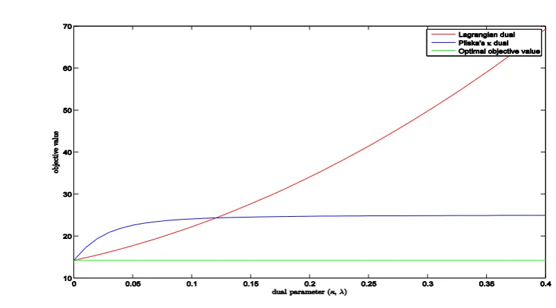
v
We can depict the objective functions of the two dual problems in the same figure. Two situations may occur according to different returns of risky security, R. Figure 1 represents the situation when the optimal Lagrangian multiplier
* is bigger than zero. In such a situation,
* and the corresponding dual parameter*
Figure 1: Situation with optimal parameters bigger than 0
Figure 2 illustrates the situation when the optimal Lagrangian multiplier
* equals to zero. In such a situation, both
* and the corresponding parameter
* are equal to zero, and the optimal objective values of the lagrangian dual and the Pliska’s dual are still equal to the optimal objective value of the primal problem.Figure 2: Situation with optimal parameters equal to 0
Example 2. Consider Example 5.11 in [1] which is a two-period problem with short-selling prohibited, the bond return rate given as
r
1
r
1
and the price process for the single risky asset and the probability measure specified as follows:
0
( )
1( )
P()1
8/5 9/8 1/42
8/5 6/8 1/43
4/5 6/4 1/44
An investor with a log utility function, U(V)=ln(V), enters the financial market with initial wealth v=1. The optimal dual parameter , trading strategies and wealth process have been derived in [1]. More specifically, the corresponding optimal process
* is* * *
0 1 1 2 1 3 4
1
0,
({ ,
})
,
({
,
})
0,
16
and the optimal trading strategies are* * *
0 1 1 2 1 3 4
5
2
,
({ ,
})
0,
({
,
})
,
3
3
yielding the corresponding optimal terminal wealth process as1 1 2 1 3 4
2
({ ,
})
2,
({
,
})
,
3
V
V
2 1 2 2 2 3 2 4
1
(
)
2,
(
)
2,
(
)
1,
(
)
.
2
V
V
V
V
Solving the Lagrangian dual problem,
min max
E ln V
( (
2))
0 0
1({ ,
1 2})
1({ ,
1 2})
1({
3,
4})
1({
3,
4}),
gives rise the optimal Lagrangian parameter process,
*,* * *
0 1 1 2 1 3 4
1
0,
({ ,
})
,
({
,
})
0.
64
It can be verified that the optimal trading strategies derived from the Lagrangian dual and Pliska’s dual are exactly the same, and, furthermore, (6) holds.
V. CONCLUSION
By identifying the relationship between the Lagrangian dual and Pliska’s dual for the constrained portfolio selection problem, we have derived in this paper a guaranteed strong duality result for a class of discrete-time constrained convex portfolio selection problems. More specifically, we ensure the existence of an optimal in the strong duality conditions of [1] to guarantee the success of the risk neutral computational approach.
The authors declare that there is no conflict of interests.
REFERENCES
[1] S. R. Pliska, Introduction to Mathematical Finance: Discrete Time Models, Blackwell, Oxford, UK, 1997. [2] J. Cvitanic and I. Karatzas, Convex duality in constrained portfolio optimization, The Annual of Applied
Probability, 2(1992), 767–618.
[3] G. L. Xu and S. E. Shreve, A duality method for optimal consumption and investment under short-selling prohibition. i. general market coefficients, The Annals of Applied Probability, 2(1992), 87–112.
[4] G. L. Xu and S. E. Shreve, A duality method for optimal consumption and investment under short-selling prohibition. ii. Constant market coefficients, The Annals of Applied Probability, 2(1992), 314–328. [5] J. C. Cox and C. F. Huang, Optimal consumption and portfolio policies when asset prices follow a
diffusion process, Journal of Economic Theory, 49(1989), 33–83.
[6] R. T. Rockafellar, Convex Analysis, Princeton, NJ: Princetion University Press, (1970).
[7] J. Harrison and D. Kreps, Martingales and multiperiod securities markets, Journal of Economic Theory, 20(1979), 381–408.
[8] J. Harrison and S. Pliska, Martingales and stochastic integrals in the theory of continuous trading, Stochastic Process, 11(1981), 215–260.