Application Of Laplace Transform To Pressure
Transient Analysis In A Reservoir With Internal
Circular Boundary
Nmegbu, Chukwuma Godwin Jacob, Olaleye, Oluwaseun .E, Pepple, Daniel .D
Department of Petroleum Engineering, Rivers State University of Science and Technology, Port Harcourt, Nigeria; Email: [email protected]
ABSTRACT: A practical pressure transient analysis method is presented for a drawdown test in a well near a constant pressure internal circular boundary. The problem was mathematically posed and solved using the Laplace Transformation with the Laplace solutions presented in this work. Internal boundaries are viewed as circles with infinite radii and act as a known limiting case for finite radii internal boundaries. The time it takes pressure transient to reach the internal circular boundary and the permeability of the reservoir formation bounded by an internal discontinuity is estimated using generalized type curves. Using a new generalized type curve developed in this investigation, the bounded reservoir permeability and transient time to the internal boundary was determined by generalized semi-log type curve matching without using the usual double straight line technique
Keywords:Pressure transient, Laplace transform, internal circular boundary, Drawdown test, Type curves
1
I
NTRODUCTIONReservoir with constant pressure internal circular boundaries occurs naturally in oil fields as gas caps and in geothermal fields as steam or non-condensable gas caps. Mangold et al. (1981) studied the effects of a thermal discontinuity on well test analysis in geothermal reservoirs [1]. These boundaries can also be induced artificially during steam flooding, in- situ combustion, immiscible gas drive, aquifer gas storage and growth of steam or gas bubbles below the bubble point pressure. A stimulation program, such as acidizing, can also result in a permeability discontinuity [2], [3]. Wattenburger and Ramey (1970) as reported in [3], [4], [5] treated a finite thickness skin region as a composite system. In any of these cases, testing a well completed in the liquid zone, exterior to the circular discontinuity, can provide estimates of permeability of the reservoir section within this internal sub-region, time taken for pressure transient to reach it and the distance to it using, diffusivity equation, numerical Laplace transform and a generalized semi-log type curve. In recent years, the numerical Laplace transformation of initial boundary value problems has proven to be useful for well test analysis applications. However, the success of this approach is highly dependent on the algorithms used to perform the numerical inversion. For this inversion, the Stehfest’s algorithm (1970) is normally used and included in conventional software applications in the oil industry. Stallman in 1952 published log-log type curves for both the no-flow and constant pressure linear boundaries. His curves are applicable for the analysis of single well tests and also for interference tests. (Raghavan, Meng, and Reynolds in1980) presented a new procedure to analyze pressure buildup data following a short flow period by utilizing drawdown type curves [6]. This research used a pressure-rate drawdown data in the transient analysis of the reservoir with internal circular boundary induced by non-condensable gas caps. Drawdown type curve including storage and skin was first published by Agarwal, Al-Hussainy, and Ramey, in 1970. These type curves allow a graphical method of determining reservoir parameters; but, more importantly, allowed a description of the reservoir/well system model [7]. The most recent advances in type curve matching and analysis came from Bourdet et al in 1983 with the introduction of derivative
type curves. Following the earlier concepts of finding the slopes of the semi-log plots, derivative type curves are plots of the derivative of the semi-log curve plotted on a log-log scale. Derivative curves allowed for determination of the reservoir parameters like skin, permeability, e.t.c., as well as the identification of well and reservoir flow behavior [8]. The thrust of this research is to develop a pressure transient analysis method for a drawdown constant rate test for a well near an internal circular boundary. This reservoir limit test may be analyzed to determine permeability of the reservoir section within the discontinuity and the transient time it takes to reach the circular discontinuity. Also, this research is aimed at using Laplace transform to further simplify the differential diffusivity equation describing fluid flow through a reservoir system with an internal circular boundary, developing a general analytic solution in Laplace space to determine wellbore pressure, pressure transient distribution and their time rate of change in the considered reservoir system and finally to determine the effects of internal reservoir limits on the pressure response of a well, permeability of the reservoir section within the discontinuity and the transient time to the internal circular boundary. The generated generalized semi-log type curve is derived from the diffusivity equation with the imposed boundary conditions of a reservoir with a circular internal boundary. The equation is then solved using Laplace transforms. The resulting equation is further resolved to modify the Bessel functions. Also using Stehfest’s algorithm, the Laplace equation governing the type curve is inverted numerically
.
2.1 Model Description
Figure-1: Schematic diagram of a constant pressure wellbore system (Sageev, A (1983))
2.2 Model Development
Before applying the Laplace transform to develop the necessary pressure transient curves, the pressure P (r, Ө, t) must satisfy the following equation and boundary conditions:
(1) Hydraulic diffusivity, (2)
Initial Condition: The reservoir is initially at constant pressure (i.e. uniform pressure distribution throughout the reservoir at time zero.)
( ) (3)
Inner Boundary Condition: Depends on the production conditions at the wellbore surface (r= ). Assuming the well is produced at a constant production rate, q, for all times.
(4) Outer Boundary Condition: This condition is usually used to indicate the reservoir boundaries for infinite-acting reservoirs and is given as follows:
( ) (5) Where, 𝑐
Equation (4) is the condition at the line source well exterior to the constant pressure boundary. The derivation of Equation (4) follows;
The flow around the well is assumed radial:
( ) (6) Equation (6) is derived from
( ) (7)
Now, as R tends to 0, q(R) tends to q, so that the rate of production out of the system is maintained constant, hence Equation (4):
2.2.1 Assumptions
To develop analysis techniques for well testing several simplifying assumptions about the well and reservoir to be modeled must be made. However, the following assumptions where introduced to achieve the objectives of this work:
1.The reservoir system is of infinite radial extent.
2.It has constant thickness, constant and isotropic permeability, constant viscosity, porosity and compressibility.
3.The pressure gradients are small so that the gradient squared terms can be neglected and that the flow is isothermal.
4.The well produces at a constant flow rate.
5.The formation is horizontal of uniform thickness and homogenous on each side of the circular inner boundary. 6.Flow is radial.
7.The discontinuity is of infinitesimal thickness in the radial direction, and can be considered stationary throughout the test period.
2.2.2 Laplace Transformation of The Diffusivity Equation
Diffusivity equation treatment using Laplace transform is more efficient than the orthodox methods. If P(t) is a pressure at a point in the reservoir and a function of time, then its Laplace transformation is expressed by the infinite integral;
𝐿* ( )+ ̅( ) ∫ 𝑒 ( )Ԁ , (8) Where, constant (s) in Equation (8) is the Laplace operator or parameter.
If we treat the diffusivity equation by the process implied by Equation (2), the partial differential can be transformed to a total differential equation. This is performed by multiplying each term in Equation (2) by 𝑒 and integrating with respect to time between zero and infinity, as follows:
∫ 𝑒 *
+ Ԁ ∫ 𝑒 (
) Ԁ , (9) Since P is a function of radius and time, the integration with respect to time will automatically remove the time function and leave P as a function of radius only. This reduces the LHS to a total differential with respect to r and , given as follows; ∫ 𝑒 * + Ԁ ∫ 𝑒 Ԁ ∫ 𝑒 Ԁ ∫ 𝑒
𝑑 (10)
∫ 𝑒 Ԁ ∫ ( Ԁ ) ̅
, (11)
Similarly other part of Equation (10) LHS was transformed and yields;
*Ԁ ̅Ԁ + ̅ ∫ 𝑒
Ԁ , (12)
The RHS of Equation (9) is also transformed using the initial reservoir condition. If we consider that P (t) is a cumulative pressure drop, and that initially the pressure in the reservoir is constant everywhere so that the cumulative pressure drop, P(t)=0. Then the integration of the RHS becomes;
∫ 𝑒 Ԁ 𝑒
( ) ,
∫ 𝑒 ( )Ԁ
∫ 𝑒 ( )Ԁ , (13)
As this term is also a Laplace transform, Equation (13) becomes;
∫ 𝑒 ( )Ԁ ̅, (14) Therefore the Laplace transform of Equation (2) becomes a total differential equation given as;
̅
̅
̅
̅, (15)
̅
̅
̅
̅ , (16) The IBVP is defined by the following set of equations in the
Laplace domain:
̅ (18)
2.2.2 Laplace Transform Solution
The solution for the homogeneous boundary conditions, Equations (16), (17) and (18), in a coordinate system centered at the well is:
̅ ( √ ⁄ ) (19)
The derivation of Equation (19), see (Appendix A). By the addition theorem for Bessel Functions, (Carslaw and Jaeger 1946, pg. 377), we translate Equation (19) to a coordinate system centered at the center of the hole:
̅ ∑ cos(𝑛 )𝐼 ( √ ⁄ ) ( √ ⁄ ) for, r<
(20)
̅ ∑ cos(𝑛 )𝐼 ( √ ⁄ ) ( √ ⁄ ) for, r>
(21)
In order to satisfy the condition of constant pressure at the internal boundary, we assume that ̅ takes the following form: for r<
̅
∑ cos(𝑛 )[𝐼 ( √ ⁄ ) ( √ ⁄ ) 𝐴 ( √ ⁄ )] (22)
For r> ̅
∑ cos(𝑛 )[𝐼 ( √ ⁄ ) ( √ ⁄ ) 𝐴 ( √ ⁄ )] (23)
where the constants 𝐴 are to be set by the boundary condition. The particular solution 𝐴 is picked in order to satisfy the condition at Infinite radii. A similar method for constructing the solution to the problem of an eccentric well within a circular sub-region was presented by Carslaw and Jaeger (1946). Equations (22) and (23) can be written as: For r<
̅ ∑ 𝜀 cos(𝑛 )[𝐼 ( √ ⁄ ) ( √ ⁄ )
𝐴 ( √ ⁄ )] (24)
For r>
̅ ∑ 𝜀 cos(𝑛 )[𝐼 ( √ ⁄ ) ( √ ⁄ )
𝐴 ( √ ⁄ )] (25)
Where: For n=0, 𝜀 1 For n>0, 𝜀
The internal boundary condition determines the coefficient,
𝐴 :
𝐴 ( √ ⁄ ) ( √ ⁄ )( √ ⁄ ) (26) Substituting Equation (26) into Equations (24) and (25) yields
̅ ∑ 𝜀 cos(𝑛 ) [𝐼( √ ⁄ ) ( √ ⁄ )
( √ ⁄ ) ( √ ⁄ )
( √ ⁄ ) ( √ ⁄ )] For r<r
(27)
̅ ∑ 𝜀 cos(𝑛 ) [𝐼( √ ⁄ ) ( √ ⁄ )
( √ ⁄ ) ( √ ⁄ )
( √ ⁄ ) ( √ ⁄ )]
For r> (28)
In order to provide general solutions, the problem is non-dimensionalized for analysis using the standard dimensionless variables defined as follows:
( )
(29)
(30)
(31)
(32)
𝑎 (33)
(34)
Substituting Equations (29) through (34) into Equations (27) and (28) yields
̅̅̅
∑ 𝜀 cos(𝑛 ) [𝐼 ( √ ) ( √ )
( √ ) ( √ )
( √ ) ( √ )] (35)
For <
̅̅̅
∑ 𝜀 cos(𝑛 ) [𝐼 ( √ ) ( √ )
( √ ) ( √ )
( √ ) ( √ )] (36)
For >
Note that Equation (35) is equal to Equation (28) with and
interchanged. The Laplace solution was inverted numerically using an algorithm developed by Stehfest (1970) since an analytical inversion of the solution in Laplace space is complicated at best and impractical at worst. A description of the algorithm is presented in (Appendix B).
3.
RESULTS
3.1 Procedures for The Determination Of The Permeability and Transient Time Of a Reservoir Within An Internal Circular Boundary.
A new generalized semi-log type curve is used for the production well. An early time infinite acting period is needed in order to use this semi-log type curve. The early time log-log match to the line source curve enables us to convert pressures to dimensionless pressures. The following procedure describes the use of the generalized semi-log type curve, Figure-5:
1. Make a log-log graph of the pressure - time response using the same scales as the log-log line source type curve.
2. Match the early time part of the data to the line source curve and pick a match point. Convert all the pressures to a dimensionless form using the match point.
3. Make a semi-log graph of the dimensionless pressure – time response using the same scale as in the generalized semi-log type curve.
4. Match this curve to the semi-log type curve (The late time data deviate above the semi-log type curve and a circular inner boundary is suspected) and pick a match point of dimensionless pressure and time. Note: The transition and the late time data are the most important portion of the match.
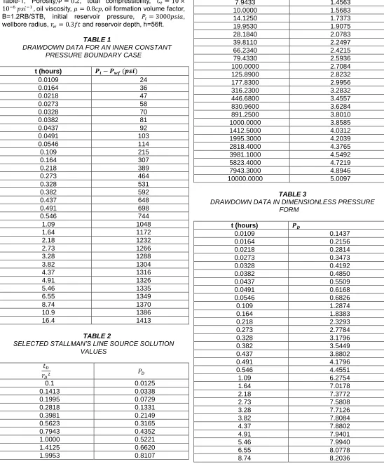
A type curve matching example is presented in this paper. The data required for analysis are hypothetical drawdown pressure – time data given by John Lee (2010) presented in Table-1, Porosity,𝛷 , total compressibility, 𝐶 1 × 1 𝑖 oil viscosity, 8𝑐 oil formation volume factor, B=1.2RB/STB, initial reservoir pressure, 3 𝑖𝑎, wellbore radius, 3𝑓 and reservoir depth, h=56ft.
TABLE 1
DRAWDOWN DATA FOR AN INNER CONSTANT PRESSURE BOUNDARY CASE
t (hours) ( )
0.0109 24
0.0164 36
0.0218 47
0.0273 58
0.0328 70
0.0382 81
0.0437 92
0.0491 103
0.0546 114
0.109 215
0.164 307
0.218 389
0.273 464
0.328 531
0.382 592
0.437 648
0.491 698
0.546 744
1.09 1048
1.64 1172
2.18 1232
2.73 1266
3.28 1288
3.82 1304
4.37 1316
4.91 1326
5.46 1335
6.55 1349
8.74 1370
10.9 1386
16.4 1413
TABLE 2
SELECTED STALLMAN’S LINE SOURCE SOLUTION VALUES
0.1 0.0125
0.1413 0.0338
0.1995 0.0729
0.2818 0.1331
0.3981 0.2149
0.5623 0.3165
0.7943 0.4352
1.0000 0.5221
1.4125 0.6620
1.9953 0.8107
2.8184 0.9660
3.9811 1.1262
5.6234 1.2900
7.9433 1.4563
10.0000 1.5683
14.1250 1.7373
19.9530 1.9075
28.1840 2.0783
39.8110 2.2497
66.2340 2.4215
79.4330 2.5936
100.0000 2.7084
125.8900 2.8232
177.8300 2.9956
316.2300 3.2832
446.6800 3.4557
830.9600 3.6284
891.2500 3.8010
1000.0000 3.8585
1412.5000 4.0312
1995.3000 4.2039
2818.4000 4.3765
3981.1000 4.5492
5823.4000 4.7219
7943.3000 4.8946
10000.0000 5.0097
TABLE 3
DRAWDOWN DATA IN DIMENSIONLESS PRESSURE FORM
t (hours)
0.0109 0.1437
0.0164 0.2156
0.0218 0.2814
0.0273 0.3473
0.0328 0.4192
0.0382 0.4850
0.0437 0.5509
0.0491 0.6168
0.0546 0.6826
0.109 1.2874
0.164 1.8383
0.218 2.3293
0.273 2.7784
0.328 3.1796
0.382 3.5449
0.437 3.8802
0.491 4.1796
0.546 4.4551
1.09 6.2754
1.64 7.0178
2.18 7.3772
2.73 7.5808
3.28 7.7126
3.82 7.8084
4.37 7.8802
4.91 7.9401
5.46 7.9940
6.55 8.0778
10.9 8.2994
16.4 8.4612
TABLE 4
SELECTED CONSTANT PRESSURE BOUNDARY GENERALIZED RADIAL FLOW TYPE CURVE VALUES
10.0000 1.6508
14.1250 1.8024
19.9530 1.9583
28.1840 2.1176
39.8110 2.2799
66.2340 2.4445
79.4330 2.6110
100.0000 2.7228
141.2500 2.8915
199.5300 3.0612
281.8400 3.2317
398.1100 3.4027
662.3400 3.5740
794.3300 3.7456
1000.0000 3.8603
1412.6000 4.0328
1995.3000 4.2015
2818.4000 4.3546
3981.1000 4.4764
6623.4000 4.5532
7943.3000 4.5915
10000.0000 4.6019
14125.0000 4.6063
19953.0000 4.6059
28184.0000 4.6053
39811.0000 4.6050
66234.0000 4.6050
79433.0000 4.6051
100000.0000 4.6051
141250.0000 4.6052
199530.0000 4.6052
281840.0000 4.6052
398110.0000 4.6052
662340.0000 4.6052
794330.0000 4.6052
1000000.0000 4.6052
1412500.0000 4.6052
1995300.0000 4.6052
2818400.0000 4.6052
3981100.0000 4.6052
6623400.0000 4.6052
7943300.0000 4.6052
10000000.0000 4.6052
3.2 Validation Of A New Type Curve Matching Method
Figure-2 is a log-log plot of the drawdown data. Figure-4 is a log match of the data to the (Stallman’s) line source log-log type curve (Shown in Figure-3). The log-log-log-log match yields a conversion factor between P and as shown in Figure-4.
The match point is:
(37)
Using (37) we convert the pressure values to dimensionless pressures and make a semi-log graph of the dimensionless pressure Vs real time as shown in Figure-5. It should be noted that the time axis need not to be converted to dimensionless form. Next, the semi-log graph of the dimensionalized drawdown data is matched to the generalized semi-log type curve (Figure-6) in Figure-7. This match concentrates on the late time data and the transition. The early time data, which do not match to the first straight line, correspond to early time line source behavior prior to a dimensionless time of 100. This early time portion of the data can be matched to the lowermost portion of the type curve. At the match point:
3 8, 3
Figure-2: Log-Log plot of drawdown data for a production well
Figure-4: Log-Log match of the drawdown data for the production well
Figure-5: Semi-log plot of the drawdown data in dimensionless pressure form.
Figure-6: Constant pressure boundary generalized radial flow semi-log type curve.
Figure-7: Semi-Log match of the drawdown data to the generalized type curve.
Finally, matching the log-log type curve of drawdown pressure-time data with the generalized semi-log type curve as shown in Figure-8. Once the fit is found by horizontal and vertical shifting, a match point is chosen to determine the relationship between actual time and dimensionless time, actual pressure drawdown and dimensionless pressure for the test being analyzed. Hence, I obtain at the match point:
3 , ( ) 𝑖, t = 0.28 hours and
Figure-8: Log-Log match of the drawdown data for the production well with the generalized radial flow Semi-Log type
curve.
Next, we solve for formation permeability, (k), the time it takes the pressure transient to reach the circular internal boundary and using the dimensionless variables definition:
(38)
1 1 (
) (39)
𝛷𝑐 ( ) (40)
Substituting the values into Equation (39),
Substituting the values into Equation (38),
× × × × ×
t = 0.19580
4 CONCLUSION AND RECOMMENDATION
In this study, a drawdown pressure transient analysis for a producing well at constant rate near an internal circular boundary was considered.. The objective of this reservoir limit pressure transient analysis method is to estimate the permeability of the formation bounded by the discontinuity and the time taken for pressure transient to reach the boundary. The conclusions represent information critical to the analysis of pressure drawdown test data and they are as follows:
Two type curves are used in this new method. The log-log type curve of the line source is used to convert the pressure data to a dimensionless form.
The new generalized semi-log type curve is used to determine the reservoir permeability and time taken for pressure transient to get to the internal circular discontinuity.
A log-log plot of Vs differs from a log-log plot of
( ) Vs t (for a drawdown test) only by a shift in the region of the coordinate system-i.e., log differs from log t by a constant and log differs from log( ) by another constant. To show this we note that;
o
o ( ) , thus
o 𝑔 𝑔 𝑔 and
o 𝑔 𝑔( ) 𝑔
The drawdown pressure response of a well near a no-flow boundary hole exhibits an infinite acting period, a transition period and a second infinite acting period.
4.1 Recommendations
To minimize error in obtained result, the plot of an actual drawdown test (log t Vs. log ) should have the a shape identical to that of a plot of log o therefore both the horizontal and vertical axes have to be displaced (i.e., shift the origin of the plot) to find the position of best fit.
Although the type curves developed here are from solutions to flow equations for slightly compressible fluid (oil), they can also be used to analyze gas well tests simply by the transformation of the flow equations to model the gas flow in terms of pseudo-pressure. And the comparison of these solutions expressed in terms of dimensionless pseudo-pressure with solutions of dimensionless pseudo-pressure for slightly compressible liquids. ( 𝑐 )
( 𝑐 )
NOMENCLATURE
A area [L2]
Bg gas formation volume factor [dimensionless] Bo oil formation volume factor [dimensionless]
Bw water formation volume factor [dimensionless] c compressibility [Lt2/M]
cA Dietz shape factor [dimensionless] cf fluid compressibility [Lt
2
/M]
cg gas compressibility [Lt
2
/M]
ci compressibility at initial conditions[Lt
2
/M]
co oil compressibility [Lt
2
/M]
cr rock compressibility [Lt
2
/M]
pwf flowing well pressure [M/Lt
2
]
pws shut in well pressure [M/Lt
2
]
plhr pressure at one hour [M/Lt
2
]
g unit conversion content
T Temperature
Cs wellbore storage constant [L
4
t2/M]
d distance [L]
h thickness [ft]
J productivity index [L4t2/M]
k absolute permeability [L2]
kf fracture permeability [L
2
]
kh horizontal permeability [L
2
]
km matrix permeability [L
2
]
kr r-direction permeability [L
2
]
kv vertical permeability [L
2
]
kx x-direction permeability [L
2
]
ky y-direction permeability [L
2
]
rd effective drainage radius [L] re external radius [L]
reD dimensionless external radius [dimensionless] Z gas compressibility factor [dimensionless]
P pressure [M/Lt2]
PD dimensionless pressure [dimensionless] pI initial pressure [M/Lt
2
]
tD dimensionless time [dimensionless]
tDA
dimensionless time based on area [dimensionless]
T time [t]
pD’
derivative of dimensionless pressure [dimensionless]
average reservoir pressure [M/Lt2]
dimensionless flow rate [dimensionless] dimensionless pressure drop [dimensionless]
∆te equivalent shut in time [t]
qsc flow rate at standard conditions [L
3
/t]
qsf Sandface flow rate at standard conditions [L
3
/t]
qt total flow rate qw water flow rate [L
3
/t]
qwb wellbore flow rate [L
3
/t]
REFERENCES
[1] Streltsova, T. (1984). Buildup analysis for interference tests in stratified formations . Journal of Petroleum Technology.
[2] Tempelaar-Weitz, W. (1961). Effect of oil R
production rate on performance of wells producing from more than one horizon . Society of Petroleum Engineers Journal.
[3] W.Hurst, A. V. (1949). Application of Laplace transform to flow problems in reservoirs. Journal of Petroleum Technology.
[4] Woods. (1970). Pulse test response of a two zone reservoir . Society of Petroleum Engineers Journal.
[5] Yasin, I. B. (2012). Pressure Transient Analysis Using Generated Well Test Data from Simulation of Selected Wells in Norne Field.
[6] Raghavan, R., Meng, H., and Reynolds, A.C. Jr., "Analysis of Pressure ... of the pD Function to Interference Analysis," J. Petroleum Technology, August 1980.
[7] Adams, A. R., H. J. Ramey, and R. J. Burgess, “Gas Well Testing in a Fracture Carbonate ...
Agarwal, R. G., R. Al-Hussainy, and H. J. Ramey, Jr. (1970).
[8] Bourdet, D. P., Whittle, T. M., Douglas, A. A., & Pirard, Y. M. (1983). A new set of type curves simplifies well test analysis (pp. 95-106).
[9] Richard, S. (1998). Reservoir Contiunity. In S. Richard, Element of Petroleum Geology (Second Edition) (p. 281). London: Academic Press.
[10]Knipe, R. J.; Jones, G.; Fisher, Q. J. (1998). Faulting, Fault Sealing and Fluid Flow in Hydrocarbon Reserviors: An Introduction. London, Special Publications (pp. i-xxi). London: Geological Society, London, Special Publications.
[11]Dake, L. P. (2001). Appraisal Well Testing. In L. P.
Dake, THE PRACTICE OF RESERVOIR
ENGINEERING (REVISED EDITION) (pp. 147-151).
[12]Horner, D. .. (1951). Pressure Buiid-UP in Wells.
Third World Petroleum Congress, Sec. II (pp. 503-521). Netherlands: D. J. Brill, Leiden.
[13]Jones, P. (1962). Reservoir Limit Test on Gas Wells. Journal of Petroleum Technology, 613-619.
[14]Davis, E. G., & Hawkins, M. F. (1963). Linear Fluid-Barrier Detection by Well Pressure measurements. Journal of Petroleum Technology, 1077-1079.
[15]Gray, K. E. (1965). Approximating Well-to-Fault Distance from Pressure Build-up Tests. Journal of Petroleum Technology, 761-767.
[16]Dorothy, G. (1998). A Direct Method for Determination of No-Flow Boundaries in Rectangular Rerservoirs Using Pressure Buildup
Data. A Direct Method for Determination of No-Flow Boundaries in Rectangular Rerservoirs Using Pressure Buildup Data. Edmonton, Alberta, Ottawa, Canada: National Library of Canada.
[17]Abraham, S. (1983, June). Pressure Transient Analysis of Reservoirs with Linear or Internal Circular Boundaries. SGP-TR-65. Stanford, California, United States of America: Stanford Geothermal Program Interdisciplinary Research in Engineering and Earth Sciences STANFORD UNIVERSITY.
Appendix A
Derivation of Pressure Transient Distribution Equation in Laplace Domain
̅
̅
̅
̅
(1) ̅
̅
̅
̅ (2)
̅( )
(3)
̅
(4) From Abramowitz and Stegun, Handbook of mathematical Functions, (Page 374, Equation 9.6.1 given by;
𝑧
(𝑧 𝑣 )𝑤
(5)
Equation 5 general solution is expressed as;
𝑤 𝐴 (𝑍) 𝐵𝐾 (𝑍)
(6) Where, (𝑍) 𝑎𝑛𝑑 𝐾 (𝑍) are Bessel functions of the first and second kinds respectively. Comparing Equations (2) and (5). We recognize that equation (1) as the modified Bessel’s equation equation of order zero which yields the general solution of the diffusivity equation written directly from Equation (6) as;
̅( ) 𝐶 (𝑍) 𝐶 𝐾(𝑍) (7) Where ̅( ) is the Laplace transform of P(t)
Let, Z = √( )R
(8) Substituting Z into equation (7) yield
̅( ) 𝐶 (√ ) 𝐶𝐾 (√ ) (9) The constants in equation (9) are obtained from the boundary conditions. The outer boundary condition represented by equation (3) indicates that 𝐶 (𝑏𝑒𝑐𝑎 𝑒 𝑥 (𝑥) and equation (3) is satisfied only if 𝐶 Therefore,
̅( ) 𝐶𝐾 (√ ⁄ ) (10) From Equation (8) to (15), we obtain
( ̅ ) 𝐶 (√ ) 𝐾 [√ ]
(11) Re-writing Equation (11)
𝐶 (√ ) 𝐾 [√ ]
(12)
Making 𝐶 the subject formula yields;
𝐶
̅( ) √
(√ ) [√ ] (14)
To complete the solution of the problem, equation (14) should be inverted back to the real time domain, the real time inversion of equation of equation (14), however is available in terms of standard function. One option is to use the Stehfest’s numerical algorithm. Another option is to find an appropriate inversion. One of these asymptotic forms is known as the line-source solution and commonly used in PTA. To obtain the line-source approximation of the solution given in equation (16), we assume that radius of the wellbore is small compared with the other dimension of the reservoir. Thus, if we assume
and use the relationship given in equation (12), we obtain
(𝑍) 1 (15)
√ ( ) 𝐾 [√ ( ) ] 1
Using this relation in equation (16), we obtain the line-source solution the Laplace domain as;
̅( ) √ (16)
Appendix B
******Stehfest (Laplace transforms numerical inversion method) ******
Public Function Li (ByVal k As Integer) As Double Dim i As Integer
Li = 1
For i = 2 To k Step 1 Li = Li * i
Next i End Function
Public Function Vi (ByVal i As Integer, ByVal n As Integer) As Double
Dim j, k, min As Integer
Dim M As Double j = Int ((i + 1) / 2) M = 0
If i <= (n / 2) Then min = i Else min = (n / 2) For k = j To min Step 1
Vi = (k ^ (n / 2) * Li (2 * k)) / (Li (n / 2 - k) * Li (k) * Li (k - 1) * Li (i - k) * Li (2 * k - i))
M = M + Vi Next k
Vi = (-1) ^ (n / 2 + i) * M End Function
****** (The calculations of Ei (x) function) ******
Public Function Ei (ByVal x As Double) As Double Dim x2, x3, x4, x5 As Double
Dim MM, NN As Double
x2 = x * x, x3 = x2 * x, x4 = x3 * x, x5 = x4 * x If x > 1# Then
MM = 0.2677737343 + 8.6347608925 * x + 18.059016973 * x2 + 8.5733287401 * x3 + x4
NN = 3.9584969228 + 21.0996530827 * x + 25.632956486 * x2 + 9.5733223454 * x3 + x4
Ei = Exp(-x) * MM / (x * NN) Else
x = Abs(x)
Ei = -Log(x) - 0.57721566 + 0.99999193 * x - 0.24991055 * x2 + 0.05519968 * x3 - 0.00976003999 * x4 + 0.00107857 * x5 End If