Adaptive DOA Estimation in MIMO Radar based on Canonical Correlation Analysis Method

Adaptive DOA Estimation in MIMO Radar based

on Canonical Correlation Analysis Method

Zhifeng Gao

Harbin Institute of Technology, Automatic Test and Control Institute, Harbin, China Shandong University, Department of Mechanical, Electrical and Information, Weihai, China

Email: [email protected]

Xiyuan Peng and Yu Peng

Harbin Institute of Technology, Automatic Test and Control Institute, Harbin, China Email: [email protected], [email protected]

Abstract—In multiple-input multiple-output (MIMO) radar, independent waveforms are transmitted from different antennas, and the target parameters are estimated via the linearly independent echoes from different targets. Several adaptive approaches are directly applied to target angle and target amplitude estimation, including Capon, APES (amplitude and phase estimation). The CCA (canonical correlation analysis) approach is first proposed to estimate target locations which has high peak amplitudes, then a gradient-based algorithm is presented to improve the target angle estimation accuracy based on CCA approach without spectrum peak searching. With an initial angle, the angle sequence is iteratively updated with adaptive steps and converges to local peaks which indicate the target locations. Simulations show that the target angle accuracy is improved, and the common DOA (direction-of-arrive) problem is avoided.

Index Terms—parameter estimation, multiple-input multiple-output, gradient function, adaptive step

I. INTRODUCTION

The multiple-input and multiple-output (MIMO) radar works with multiple antennas to achieve high-resolution spatial spectrum estimation and to resist the target’s scintillations (see [1,2,3] and the references).

With multiple targets application of the MIMO radar system, linearly independent waveforms are transmitted simultaneously from different antennas, these waveforms are linearly combined at the targets with different phase factors. The reflected signals from targets are received with different antennas, which are independent of each other. Several well-known adaptive approaches which have sharp peaks and high resolution, are applied to estimate the target locations and target amplitudes, including Capon [4,5] (also known as minimum variance distortionless response (MVDR)[6]), APES (amplitude and phase estimation) algorithms [7] and CAPES (combined Capon and APES) [8].

The canonical correlation analysis (CCA)[9] and the Capon spectral estimators are proved to belong to the nonparametric matched-filterbank (MAFI) class[10,11], and applied into magnitude squared coherence (MSC) [12,13] spectral estimation. Similar with the application of the Capon approach in MIMO radar, we apply the

CCA approach to multiple target locations and target amplitudes estimation from the echo waveforms, and higher target amplitudes are achieved.

Under the MAFI theory[10], the spatial spectrum is estimated on a predefined angle grids and following with local spectral peak search, and suffered with the common direction of arrival (DOA) mismatch [3,12] problems in beamforming applications.

To avoid the common DOA problem and improve the estimation accuracy, a scalar cost function is developed based on the denominators of the CCA spatial spectrum, and the local minimum of the cost function indicates the target location. A gradient-based adaptive-step algorithm (will be referred as SITER algorithm) is presented. With an initial angle, an angle sequence is iteratively updated and converges to local minimum point. High accuracy and high peak amplitude are achieved.

For multiple target parameter estimation, the cost function has several local minimum points. An angle selection strategy is developed where the initial angles are iteratively selected and the needless duplications are avoided. The strategy is applied with SITER algorithm and the algorithm (will be referred as AITER algorithm) to find all the local minimum points is developed.

The SITER and AITER algorithm also can be applied to adaptive DOA estimation. The estimated target angles are applied as the initial angles iteratively to obtain new target locations. The DOA angles are estimated with high accuracy, and the computations are saved.

II. PROBLEM DEFINATION

A MIMO radar system simultaneously transmits N linearly independent waveformssn =[ ,sn,1 sn,2, ," sn L, ]T ,

1, ,

= "

n N by N linear transmitting antennas, and received with M receiving antennas, where superscript T denotes the transpose, L is the snapshot number.

Letθ be the DOA angle of a far field target, and let

1

( )θ _∈ N×

t

a C be the corresponding steering vector for the transmitting antenna array. The reflected waveform vector at θ is denoted as ( )ST θ

t

and the waveforms from targets at different locations are linearly independent of each other.

The received data matrix of the receiving array is X= ( ) ( ) ( )S+Zθ μ θ T θ

r t

a a , (1) where each column of matrixX=[x ,x , ,x ]1 2 " L ∈CM L× is a

snapshot, vector _{( )θ ∈} M×1 r

a C is the steering vector of the receiving antenna array, ( )μ θ denotes the complex amplitude of the reflected signals from the target at angle

θ, matrix Z denotes the noise matrix.

Then the target parameter estimation problem is to estimate the complex amplitude ( )μ θ on each angle θof interest from the data matrix X, and the DOA angles are estimated based on the peak search of ( )μ θ .

A. The Capon Approach

Based on MAFI theory, the matched-filter _{g( )θ ∈} M×1 C is equal to solve an optimal problem

g( ) ˆ

min g ( )Rg( ) s.t. g ( ) ( ) 1

θ = θ θ θ θ =

H H

r

J a , (2)

where superscript H denotes the conjugate transpose and matrix ˆR=1/ XX⋅ H

L denotes the sample covariance matrix of the observed snapshots.

The solution is obtained by solving (2) :

1

1

ˆR ( )

ˆg ( ) _ˆ

( )R ( )

θ θ θ θ − − = r Capon H r r a

a a , (3) The output of the matched-filter can be written as

1

1

ˆ ( )R Z

ˆg ( )X ( ) ( )S+ _ˆ

( )R ( )

θ θ μ θ θ θ θ − − = H

H T r

Capon r H

r r

a a

a a (4) Applying the LS method, the estimate of complex amplitude ( )μ θ is obtained

1 *

1 *

ss

ˆ

( )R XS ( )

ˆ ( ) _{ˆ ˆ}

[ ( )R ( )][ ( )R ( )]

θ θ

μ θ

θ θ θ θ

−

−

= rH H t

Capon _{H T}

r r t t

a a

L a a a a , (5)

where superscript * denotes the conjugate transpose, and matrix ˆR =1/ SSss L⋅ H is the correlation matrix of the

transmitting waveforms. B. The APES Approach

The matched-filter g( )

θ

is equal to an optimal problem

g( )

min g ( )Qg( ) s.t. g ( ) ( ) 1

θ = θ θ θ θ =

H H

r

J a , (6)

where ₂ * _*

ss

XS ( ) ( )SX

ˆ

Q( ) R _ˆ

( )R ( )

θ θ

θ

θ θ

= − H t Tt H

T

t t

a a

L a a .

The solution is obtained by solving (6) :

1

1

Q ( ) ( )

ˆg ( )

( )Q ( ) ( )

θ θ θ θ θ θ − − = r APES H r r a

a a , (7)

The estimate of complex amplitude ( )μ θ is obtained

1 *

1 *

ss

( )Q ( )XS ( )

ˆ ( ) _ˆ

[ ( )Q ( ) ( )][ ( )R ( )]

θ θ θ

μ θ

θ θ θ θ θ

−

−

= rH H t

APES H T

r r t t

a a

L a a a a (8)

C. The CCA Approach

Under the MAFI theory, the typical matched-filters are formulated in a unified form [12], the CCA spectral estimator [9] are obtained with the optimal problem

1/2

g( ) ˆ

min g ( )R g( ) s.t. g ( ) ( ) 1

θ θ θ θ θ

−

= H H =

r

J a , (9)

The solution is obtained by solving (9) :

1/2

1/2

ˆR ( )

ˆg ( ) _ˆ

( )R ( )

θ θ θ θ − − = r CCA H r r a

a a , (10) The estimate of complex amplitude ( )μ θ is obtained

1/2 *

1/2 *

ss

ˆ

( )R XS ( )

ˆ ( ) _{ˆ ˆ}

[ ( )R ( )][ ( )R ( )]

θ θ μ θ θ θ θ θ − − = H H r t

CCA H T

r r t t

a a

L a a a a (11)

D. The Capon and CCA Spatial Spectrum

The corresponding spatial spectrum of angle θ is estimated by the output power _P( ) g ( ) Rg( )θ =ˆH θ ˆˆ θ of the

matched-filters. Then Capon and CCA spatial spectra are derived as

1

capon 1

ˆ ˆ ˆg ( )R R ( )

( ) _ˆ

( )R ( )

θ θ

θ

θ θ

−

−

= H r

H

r r

a P

a a 1

1 ˆ ( )Rθ − ( )θ

= H

r r

a a , (12)

1/2 1/2

cca 1/2 1/2

ˆ ˆ

( ) R _ˆ R ( )

( ) _ˆ R _ˆ

( ) R ( ) ( )R ( )

θ θ

θ

θ θ θ θ

− −

− −

= rH r

H H

r r r r

a a

P

a a a a

1/ 2 2

ˆ

[ ( )Rθ − ( )]θ

= H

r r

M

a a (13)

III. ITERATIVE SEARCH OF SPECTRAL PEAKS

Consider a MIMO radar system where a uniform linear array (ULA) with N transmitting antennas and M receiving antennas. The steering vectors of angle θ are defined as below

( )

_{θ =[1,} −j2 sinπd ( )θ λ/ _{, ,"} −j2 ( 1) sinπN− d ( )θ λ/ _]T t

a e e (14)

( )

_{θ =[1,} −j2 sinπd ( )θ λ/ _{, ,"} −j2 (πM−1) sind ( )θ λ/ _]T r

a e e (15)

where d denotes the space between adjacent antennas and

λ

denotes the wavelength of the waveforms. A. Gradient-based Updating Formula

Based on the denominator of CCA spatial spectrum (13), a scalar cost function in unified form is defined as

-1/2

ˆ ( )θ = H( )Rθ ( )θ

r r

J a a , (16)

1 θ ( 1), 1,2,

θm=θm− − ∇γm J θm− m= ", (17) where θm denotes the estimated DOA angle at the mth

iteration, γm is the adaptive step and ∇θJ(θm−1)is the

gradient function of the cost function ( )J θ at θm₋₁, and

the initial angleθ0 is selected with a selection strategy in

the following AITER algorithm. B. Gradient Function

The gradient function of vector ( )ar θ is defined as

( )

₁ 2 sin( )/ 2 ( 1) sin( )/

[ , π θ λ, , π θ λ]

θ

θ θ θ θ

− − −

∂ ₌ ∂ ∂ ∂

∂ ∂ ∂ " ∂

j d j M d

r T

a e e

( )U ( )θ θ

= jA ar , (18)

whereU=diag([0,1, ,"M−1])is a diagonal matrix and ( )θ = −2π cos( )/θ λ

A d is a real scalar.

Then the gradient function of ( )J θ is derived as

( )

( )

_Rˆ 1/2 _{( )}

( )

_Rˆ 1/2 ( )

θ θ _θθ − θ θ − _θθ

∂ ∂

∇ = +

∂ ∂

H

r H r

r r

a a

J a a

(

ˆ 1/2 ˆ-1/2

)

( )θ ( )U Rθ − ( )θ ( )R U ( )θ θ

= ⋅ − H + H

r r r r

A ja a ja a

(

ˆ 1/ 2

)

( ) 2Imθ ( )URθ − ( )θ

= ⋅ H

r r

A a a (19)

and∇_θJ( ) 0θ = is satisfied on each local minimum point.

C. Adaptive Step

The adaptive step γm is obtained with the optimal

problem where the cost function reached the minimum value at angle θmalong direction −∇θJ(θm−1)

1 1

( ) min ( _θ ( ))

γ

θ = θ − − ∇γ θ −

m

m m m m

J J J (20)

Based on (15) (17) and the linear approximation, the exponent function_e−j2πkdsin(θm)/λis reformulated as

1

2 sin( )/ 2 sin( )/

1 1

[1 ( ) ( )]

π θ λ π θ λ θ θ γ θ − − − − − = − ∇ m m

j kd j kd

m m m

e jkA J e

Then the steering vector ( )ar θm is reformulated as

1 1 1

( ) [Iθ = − (θ − )γ ∇θ (θ − )U] (θ −)

r m m m m r m

a jA J a (21)

where matrix I is a unit matrix with dimension M. Based on (16) (21), a closed form of ( )J θm is derived

-1/2

ˆ

( )θ = H( )Rθ ( )θ

m r m r m

J a a

-1/2

1 ˆ 1

(θ −)R (θ−) = H

r m r m

a a

-1/2

1 1 1 ˆ 1

(θ −)γ _θ (θ − ) (θ −)UR (θ −)

+ ∇ H

m m m r m r m

jA J a a

-1/2

1 1 1 ˆ 1

(θ −)γ θ (θ −) (θ −)R U (θ − )

− ∇ H

m m m r m r m

jA J a a

2 2 2 -1/2

1 1 1 ˆ 1

(θ −)γ θ (θ − ) (θ −)UR U (θ − )

+ ∇ H

m m m r m r m

A J a a

Then substitute (19) into ( )J θm , there is

-1/2 2

1 ˆ 1 1

( )θm = rH(θm−)R r(θm−)− ∇γm _θ (θm−)

J a a J

2 2 2 -1/2

1 1 1 ˆ 1

(θ − )γ θ (θ −) (θ − )UR U (θ −)

+ ∇ H

m m m r m r m

A J a a (22)

The gradient function∇γmJ( )θm is derived from (22),

( ) ( )/

γ θ θ γ

∇_mJ m = ∂J m ∂ m

(

)

2 2 -1/2

1 1 1 ˆ 1

( ) 1 2 ( ) ( )UR U ( )

θ θ − γ θ − θ − θ −

= −∇ − H

m m m r m r m

J A a a ,

where 2 1

( ) 0

θ θ −

∇ J m > is satisfied(otherwise local minimum

is reached with ∇θJ(θm−1) 0= ), the adaptive step is

calculated from∇γmJ( ) 0θm = ,

2 -1/2

1 1 1

1 ˆ

2 ( ) ( )UR U ( )

γ

θ − θ − θ −

=

m H

m r m r m

A a a (23)

Since the matrix ˆR is positive definite and invertible, -1/2

and the vectorU (ar θm−1) is non-zero vector for any angle 1

θm− ,it is clear that

-1/2

1 ˆ 1

(θ −)UR U (θ −) 0>

H

r m r m

a a . But

2 1

(θm−)

A is in the denominator of (23), all the element in angle sequence θ θ θ0, , ,1 2 "could not be θ −1= ±90

D

m with

1

(θm− ) 0=

A . In simulations, the angle interval to detect the target will be selected asθ∈ −( 90 ,90 )D D _{, the adaptive}

step is a finite positive scalar.

IV. ALGORITHM DEVELOPMENT

Based on (17)(19)(23) and starts with a given initial angle θ0 ,an angle sequenceθ θ θ0, , ,1 2" is iteratively

generated and converges to the corresponding single local minimum of function ( )J θ .

(

)

1 1

1/ 2

1 1 1 1

2 -1/2

1 1 1

1 1

( ) 2 cos( )/

ˆ

( ) ( ) 2Im ( )UR ( )

1 ˆ

2 ( ) ( )UR U ( )

( ) θ θ θ π θ λ θ θ θ θ γ θ θ θ θ θ γ θ − − − − − − − − − − − − = − ⎧ ⎪ ∇ = ⋅ ⎪ ⎪ ⎨ = ⎪ ⎪ ⎪ _{= − ∇} ⎩ m m H

m m r m r m

m _H

m r m r m

m m m m

A d

J A a a

A a a

J

(24)

Property 1: The cost function ( ) 0J θm > is monotonous

decreasing, that isJ( )θm ≤J(θm−1).

Proof: The adaptive step γm is obtained with the

optimal problem (20), where J( )θm ≤J(θm−1)is satisfied.

And it is obviously that ( ) 0J θm > with a positive matrix -1/2

ˆR and non-zero vector ( )ar θm .

Property 2: If ∇θJ( ) 0θ0 < is satisfied on initial angleθ0,

the angle sequence is monotonous increasing,θm >θm−1,

otherwise it is monotonous decreasing ,θm<θm−1.

This property will be used to select initial angles and to skip all the angles with the same local minimum point.

Property 3: With the initial angleθ0, the angle sequence

0, , ,1 2

θ θ θ " converges to the corresponding local minimum ˆθ, where∇θJ( ) 0θˆ = is satisfied.

Proof: With property 1, the cost function J( )θ is

monotonous decreasing with lower boundJ( ) 0θ ≥ , the angle sequence converges to the local minimum point.

Assuming 2 1

( ) 0

θ θ −

∇ J m > ,substitute (23) into(22) 2

1 1

( )θm = (θm−) 0.5− γm∇_θ (θm−)

J J J (25)

whereJ( )θm >J(θm−1)is satisfied with a positive step γm.

While there isJ( )θm =J(θm−1)at the local minimum

pointθm−1=θ , which is contrary with J( )θm >J(θm−1)

from (25), so 2 1

( ) 0

θ θ −

∇ J m = is satisfied at the local

minimum point.

A. Iterative Algorithms for Local Minimum Points

Based on Property 1,2,3 and (24), the iterative algorithm SITER is presented and applied to search a single local minimum point, which indicates the target location. The SITER algorithm is shown in Table 1. In practice, the exit criterion ∇_θJ( ) 0θ = is substituted for

||∇_θJ( ) ||θ ≤ε, such as ε=10−6and etc.

To obtain all the local minima, the most important task is to select the initial angles. A selection strategy is developed on Ω ={ | (θ θmax−θmin) / ,k K k=0, ," K−1}

whereθmax,θminare angle bounds. The ith initial angle θi,0

is selected: (1)θi,0>θi−1, (2)∇θJ( ) 0θi,0 < . Then angle

sequence θ θ θi,0, , ,i,1 i,2"is monotonous increasing and

converges to the ith local minimum angleθi, the other

angles with the same local minimum are skipped. Combining the initial angle selection strategy and the SITER algorithm, the AITER algorithm is developed. B. Adaptive DOA Estimation

In practice, the received data matrix at time instant n is denoted as X( )=[x( ),x(n n n−1), ,x(" n− +L 1)] , each column is a snapshot of the sampled receive data. The sampled covariance matrix ˆR( )=1/ X( )X ( )⋅ H

n L n n is

derived recursively as below

x( )x ( ) x( )x ( )

ˆ ˆ

R( ) =R( 1)n n− − n−L H n−L + n H n

L L (26)

The inverse matrix ˆR ( )-1

n is calculated with the matrix

inversion lemma and reformulated as below

-1 -1

-1 -1

-1

-1 -1

-1 -1

-1

ˆ ˆ

R ( 1)x( )x ( )R ( 1) ˆ

R =R ( 1) _ˆ

x ( )R ( 1)x( )

R x( )x ( )R

ˆR ( )=R

x ( )R x( )

⎧ _{− −}

− − ⎪

+ −

⎪ ⎨

− −

⎪ ₊

⎪ _{− − −}

⎩

H H

H H

n n n n

n

L n n n

n L n L

n

L n L n L

(27)

IV. SIMULATION RESULTS

A MIMO radar system with uniform linear arrays is applied to estimate the targets DOA and the reflected complex amplitudes, where half-wavelength spacing condition d=λ/ 2is both satisfied for N=10 transmitting antennas and M=14 receiving antennas.

A. DOA Estimation with CCA Method

Targets locate at { 40.2 , 25.4 , 10.3 ,10.2 ,20.5 }− D − D − D D D _,

the reflection parameterμ θ( )are{4,2,3,3,1}respectively. The received signal has L=256 snapshots and is corrupted by a zero-mean Gaussian noise with unknown covariance matrix and signal to noise ratio (SNR) is equal to 10dB.

The complex amplitudes estimated with Capon, APES, CCA algorithms on evenly predefined angle grids with an interval 0.5D _{are shown in Fig.1 and the results with}

angle interval 0.1D_{are shown in Fig.2. Then DOA angle}

are estimated by local peak search, the details of peaks are listed in Table 3 and Table 4 respectively.

TABLE 2 AITER ALGORITHM

AITER: ITERATIVE SEARCH FOR MULTIPLE LOCAL MINIMUM POINTS

Input: matrix ˆR , -1/2 Ω ={θ=(θmax−θmin) / ,k K k=0, ,"K−1},

1. initial value θˆ0=0 , i=1 2. for k=0,1, ,"K−1 do 3. θi,0=(θmax−θmin) /k K∈Ω

4. if θi,0>θi−1 and ∇θJ( ) 0θi,0 <

5. select θi,0 as initial frequency

6. call SITER algorithm , return θi

7. i= +i 1 8. end if 9. end for

Output: the local minimum frequencies θi, 1,2,...i= M

TABLE 1 SITER ALGORITHM

SITER: ITERATIVE SEARCH FOR SINGLE LOCAL MINIMUM POINTS

Input: matrix ˆR , initial angle -1/2 θ0, 1. for m = 1,2, … do

2. 1 / 2

1 1 1 ˆ 1

( ) ( ) 2 Im[ ( )UR ( )]

ω ω− θ− θ− − θ −

∇ = ⋅ H

m m r m r m

J A a a

3. if ∇θJ( ) 0θm =

4. θ θ= m and Stop

5. else

6. 2 -1/2

1 1 1

1 ˆ

2 ( ) ( )UR U ( )

γ

θ − θ − θ − =

m H

m r m r m

A a a

7. θm=θm−1− ∇γm θJ(θm−1) 8. end if

9. end for

In Fig. 1, the Capon and APES approached have higher resolution but lower peaks, and suffered with the common DOA problem, while the CCA approach has lower resolution but sharp peaks in complex amplitude estimations, the target DOA angles are estimated by the peak angles.

In Fig.2, the angle grids have a narrow interval 0.1, the peaks of APES and Capon are improved significantly, while computations are increased at the same time. The CCA approach is suitable on angle grid with fewer angles, and the corresponding computations are saved.

B. DOA Estimation with Iterative Algorithms

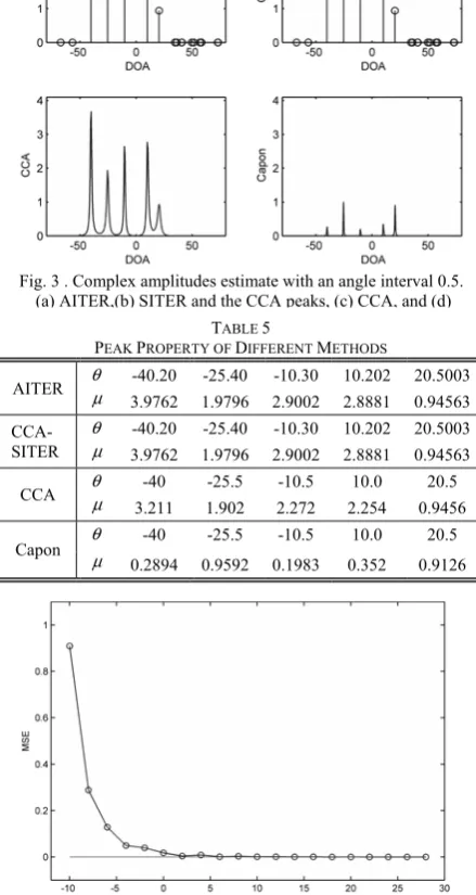
To avoid the common DOA mismatch problem, the DOA angles are estimated with the proposed iterative algorithms. The complex amplitudes of CCA and Capon approaches are shown in Fig.3(c)(d). In Fig.3 (a) the DOA angles are estimated directly with the AITER algorithm, while in Fig.3(b) the peak angles of CCA approach in Fig.3(c) are used as the initial angles of the SITER algorithm to achieve higher peaks. The details are listed in Table 5, higher estimation accuracy and higher complex amplitudes are obtained.

Fig. 4. The mean squared error of the DOA estimates versus the SNR of the reflected signal from the target

TABLE 5

PEAK PROPERTY OF DIFFERENT METHODS

AITER θ_μ -40.20 -25.40 -10.30 10.202 20.5003

3.9762 1.9796 2.9002 2.8881 0.94563

CCA-SITER θμ 3.9762-40.20 1.9796 2.9002 2.8881-25.40 -10.30 10.202 20.50030.94563

CCA θ_μ -40 -25.5 -10.5 10.0 20.5

3.211 1.902 2.272 2.254 0.9456

Capon θ_μ -40 -25.5 -10.5 10.0 20.5

0.2894 0.9592 0.1983 0.352 0.9126

Fig. 3 . Complex amplitudes estimate with an angle interval 0.5. (a) AITER,(b) SITER and the CCA peaks, (c) CCA, and (d)

TABLE 4

PEAK PROPERTY OF DIFFERENT METHODS

APES θ_μ -40.2 -25.4 -10.3 10.2 20.5

3.884 1.891 2.649 2.683 0.911

Capon θ_μ -40.2 -25.4 -10.3 10.2 20.5

3.878 1.885 2.635 2.670 0.9066

CCA θ_μ -40.2 -25.4 -10.3 10.2 20.5

3.988 1.985 2.873 2.865 0.9384

Fig. 2. Complex amplitudes estimate with an angle interval 0.1. (a) All methods, (b) APES, (c) CCA , and (d) Capon.

TABLE 3

PEAK PROPERTY OF DIFFERENT METHODS

APES θ_μ -40.0 -25.5 -10.5 10.0 20.5

0.3012 1.143 0.1465 0.294 0.911

Capon θ_μ -40.0 -25.5 -10.5 10.0 20.5

0.2869 1.114 0.1407 0.2819 0.9066

CCA θ_μ -40.0 -25.5 -10.5 10.0 20.5

3.713 1.969 2.562 2.677 0.9384

In Fig.3 (b), the DOA angles are estimated with the SITER algorithm, the initial angles is chosen to be the CCA peaks angles. The peak properties are the same between AITER and CCA-SITER algorithms. If the target number is unknown, the AITER algorithm is suitable for target location estimation.

In Fig. 4, the mean squared error (MSE) of the DOA angles of the targets are defined as _{{||θ θ}ˆ _{− || }}2

i i

E and

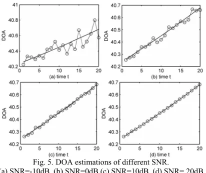
compared with different SNR. The results show that the estimation accuracy is increasing with larger SNR. C. Adaptive DOA Estimation

A target is moving across the far-field of the MIMO radar system, the initial location parameters of the target include the angle

θ

=40.24D

and the reflection parameter

( ) 4

μ θ = . The DOA angleθ( )n of the moving target is

varying about the time instant n as (28) ( ) 40.24 0.02

1,2, ,20

θ

⎧ _{= +}

⎨ = ⎩

D

"

n n

n (28) The received signal has L=16 snapshots and is corrupted by a zero-mean Gaussian noise with unknown covariance matrix and different SNR. The SITER algorithm is applied to recursively estimate the DOA angles of the moving target, where the estimated angles of time instant n-1 are used as the initial angles of time instant n , and the sampled variance matrix and the inversion matrix are calculated with (26)(27), the results are shown in Fig.5.

In Fig. 5, high estimation accuracy is achieved when SNR is large, the SITER algorithm can be easily applied in adaptive signal processing with a high accuracy and low complexity. In future, the SITER and AITER algorithms will be compared with other methods about the estimation accuracy and the computation complexity.

V.CONCLUSION

Based on MAFI theory, several nonparametric spectrum estimation methods are used for target location and target amplitude estimation. To avoid the common DOA problem and to improve the estimation accuracy, the CCA approach is proposed to DOA angle estimation,

higher peaks are achieved, but the resolution is low, and the DOA angle estimates are biased.

A gradient-based algorithm is presented to search a single local minimum, which indicates the target location. With a iteratively selected initial angle, the update angle sequence converges to the local minimum point of the cost function. An initial angle selection strategy is developed in AITER algorithm, and applied to estimate the DOA angles. The SITER algorithm is easily applied to adaptive DOA estimation and computations are saved. The results with the SITER and AITER algorithm show perfect performance of high accuracy.

ACKNOWLEDGMENT

The research presented in this paper is supported by The National Natural Science Found (61304142, 61305130).

REFERENCES

[1] H. Godrich, A.M. Haimovich, R.S. Blum, “Target Localization techniques and tools for MIMO radar” Radar Conference 2008, pp.1-6. 2008

[2] L. Xu, J. Li, “Target detection and parameter estimation for MIMO radar systems”, IEEE Trans. On Aerospace and electronic systems, vol. 44, pp. 927-939,2008.

[3] J. Li and P. Stoica, Robust Adaptive Beamforming, Wiley, New York, 2005, p.95-148.

[4] J. Capon. “High-resolution frequency-wavenumber spectrum analysis”. Proceedings of the IEEE, vol. 57, pp. 1408-1418, August 1969.

[5] R. T. Lacoss. “Data adaptive spectral analysis methods”. Geophysics, vol. 36, pp. 661-675, August 1971.

[6] J. Benesty,J. Chen,Y. Huang, “A generalized MVDR spectrum”, IEEE Signal Processing Letters. , vol. 12, pp. 827-830, December 2005.

[7] P. Stoica, H. Li, J. Li, “A New Derivation of the APES Filter”, IEEE Signal Processing Letters.vol.6(8),pp.205-206, August 1999.

[8] A. Jakobsson and P. Stoica, “Combing Capon and APES for estimation of spectral lines”, Curcuit systems signal process, vol.19, pp.159-169, 2000.

[9] I. Santamaria, J. Via. “Estimation of the magnitude squared coherence spectrum based on reduced-rank canonical coordinates”, IEEE International Conference on Acoustic, Speech, and Signal Processing. Honolulu, Hawaii, USA, April 2007.

[10]P. Stoica, A. Jakobsson,J. Li, “Matched-filter bank interpretation of some spectral estimators”. Signal Processing, vol. 66, pp. 45-59, April 1998.

[11]C. Zheng,M. Zhou,X. Li. “On the relationship of non-parametric methods for coherence function estimation”. Signal Processing., vol. 88, pp. 2863-2867, November 2008.

[12]Y. Peng, Z. Gao, X. Peng. “MVDR Spectrum estimation by dichotomous spectral peak search”, International Instrumentation and Measurement Technology conference 2012, pp.1692-1696, 2012.

[13]Y. V. Zakharov and T. C. Tozer, “Frequency estimator with dichotomous search of periodogram peak,” Electronic Letters., vol. 35, pp. 1608–1609, September 1999.

[14]J. Benesty, J. Chen,Y. Huang, “Estimation of the coherence function with the MVDR approach”, IEEE International Conference on Acoustic, Speech, and Signal Processing. Toulouse, France, May 2006.

Harbin institut areas of statis frequency estim

Xiyuan Peng engineering fr and 1992 respe

Currently, h professor, doc engineering a automatic test

Zhifeng May 27 degree i Universi M.S. de control Jinan, C Curre automati te of technolog stical signal pr mation, and dig

received B.S., rom Harbin ins

ectively. he is working i ctoral superviso and automation technology, sm

g Gao was born 7, 1979. He r in control scie ity, Weihai, Ch egree in opera theory from Sh hina in 2004. ently, he is a P

ic test and c gy. His research rocessing, spec gital filter desig

M.S. and Ph. D stitute of techno

in Harbin Instit or and dean of n. His researc mart fault diagn

n in Heze, Chin received the B nce from Shan hina in 2001 an ations research handong Unive

Ph. D student a control institu h interests are i ctral estimation gn.

D degrees in el ology in 1984,

ute of technolo f school of elec ch interests in

osis

na, on B. S. ndong nd the h and ersity,

at the ute at

in the n and

lectric 1987

ogy as ctrical nclude

Yu Peng rece degrees from H in 1996, 1998 Currently, h Harbin institut interests inclu test informatio Dr. Peng Instrumentatio

eived B.S., M Harbin institute and 2004 respe he is working

te of technolog ude modern te on processing, W

is a memb on and Measure

M.S. and Ph. D e of technology ectively.

as professor in y. His research est technology, WSNs.

ber of IEEE ment Society.

D y

n h ,