Influence Spreading on Complex Networks Effects of Node Activity and Paths with Loops

e-ISSN: 2278-067X, p-ISSN: 2278-800X, www.ijerd.com

Volume 14, Issue 4 (April Ver. I 2018), PP.01-18

Influence Spreading on Complex Networks

–

Effects of Node

Activity and Paths with Loops

Vesa Kuikka

Finnish Defence Research Agency, PO BOX 10, Tykkikentäntie 1, FI-11311 Riihimäki, Finland Corresponding Author: Vesa Kuikka

ABSTRACT: We present a method of calculating measures for centrality and betweenness in complex networks based on properties of spreading processes on networks. The model is designed for influence spreading and other similar processes. The modelling is based on temporal spreading in a topological network structure via all the possible paths from source nodes to target nodes. The contributions of different paths to the measures are computed and dependencies of the paths are taken into account using probability theory. The method is not limited to network structures near the source nodes, instead, the measures can be calculated for different sizes of networks. When the spreading process is modelled with time dependencies, weighting factors describing the activity of nodes is an essential aspect of the theory. Typically, the measures for passive and active networks have different values, for example, rankings of the most influential nodes may not be the same. Furthermore, we show how to model processes where revisits along different routes are allowed. The method is demonstrated along the lines of an artificial network designed for illustrations. After that the method is also applied to a real-world social network.

KEYWORDS: Social Networks, Centrality Measure, Closeness Centrality, Betweenness Centrality, Influence Measure, Network Topology, Influence Spreading, Node Activity, Temporal Spreading Distribution.

--- --- Date of Submission: 22-03-2018 Date of acceptance: 05-04-2018 --- ---

I.

Social, technical, and biological networks have been a widely studied area in the general theory of networks. In social networks community structures are an important field of research due to general globalization and increased networking in societies. Many applications in social sciences exist and, on the other hand, network analysis in support of the overall security, like the investigation of terrorist groups and connections between their members has become a topical subject. In this paper, we present a new method for measuring the influence, information, and rumour spreading in social or technical networks [47]. Albeit the general method can be used for different kinds of spreading processes, we use often the term “influence spreading” in this paper. After all, much of the research of complex networks concern social networks and influence spreading. The measures can be used as influence measures, or more generally, as “spreading measures”. The method serves as basic ground work for investigating more detailed spreading models and measures in sociological, technical, epidemic [39], and biological networks.

Interactions in social networks have been studied to understand the spreading of attitude or opinion changes, formation of sub-groups, and organizational issues. Herbert Kelman [29] has investigated how people influence one another. He described three types of opinion change: compliance, identification and internalization. Later, more advanced theories have been presented but Kelman’s categorization indicates that different forms of interactions exist and in detailed sociological models these should be studied. As another example, Cialdini's theory of influence is based on six key principles: reciprocity, commitment and consistency, social proof, authority, liking, and scarcity [10].

Identifying most influential nodes in social networks is important in many applications [3], [4], [9], [13], [19]–[21], [25], [30], [36], [38], [43]–[46]. Several measures for ranking and measuring prominence of nodes in a network have been proposed based on centrality and betweenness [5], [6], [7], [14]. However, most of these measures lack exact definitions of the context of use and quantitative interpretation. Research has investigated influence, information, and rumour spreading with various mathematical methods [11], [12], [16], [17], [37], not all of them are based on exact topological network structures.

application. Typically the measures are local and they cannot be applied to large networks. Measures which discover the most important nodes in a network do not necessarily generalize to the remaining nodes. Some development in this area has been achieved recently [1], [34]. Spreading measures defined in this paper have quantitative interpretations defined as the probability of influence of a node on another node in the network. The method relies on analytical calculation of probabilities of spreading along paths in a network and their appropriate combination in a probabilistic setting.

Stephen Borgatti [5] has considered different kinds of traffic in a network: used goods, money, gossip, e-mail, attitudes, infection, and packages. Borgatti says about attitude changes: “The notion is of an influence process in which, through interaction, individual effect changes in each other’s beliefs and attitudes. The attitudes spread through replication rather than transfer. A speaker may persuade many people at the same time, and the trajectories followed by the attitude can revisit links – I can continue to influence you about the same thing over time.” And also [15]: “In a friendship network, we expect the ties to serve as a backcloth along which traffic may flow. So if there is a path from A to B to C to D, we expect that over time and with some probability something (e.g. information) could diffuse from A to D.”

Network spreading measures have been developed using, for example, local structural characteristics [6], [7], geodesic distances [1], and random walks [40]. Geodesic distances and random walks are based on considering paths of different lengths. The concept of random-walk effective distance published in [26] can be applied to any weighted and directed network, for instance in the context of transportation, social interactions and rumour spreading. The formalism of temporal accessibility graphs has been used to analyse temporal network data in terms of causal paths [35]. An accessibility graph is built by consecutively adding paths of growing length.

In this paper, the method for calculating spreading measures is designed with some main principles in mind. Closed form exact calculations with many aspects of the theory are carried out. These include the structure of the network, the spreading distribution of influence in networks and the modelling of different node characteristics and paths in the network. In this paper, we consider spreading processes where edges of a network have no capacity limitations. The theory is based on dynamical spreading of influence as a function of time [8], [22]–[24]. In the model, the propagation proceeds in the same way regardless of the states of nodes of each path between source and target nodes. States the individual nodes could take are ‘received/not received a piece of information’. In many applications the spreading process results in the change of node states in networks. Percolation centrality measures the importance of nodes in terms of percolation states of nodes as a function of time [41].

The measures proposed are based on probabilities for an influential spreader (or spreaders) and mediator nodes to spread influence. Topological structure of a network, weighting factors describing the activity of nodes or links and temporal spreading distribution via paths in the network are used as input. Ties between nodes can be bidirectional or unidirectional. The proposed model is dynamic and it can be used for identifying key players in collective dynamics [31]. An artificial network [30] is analysed and compared with other results from the literature. The method is also applied to a real-world social network. Rankings of nodes can change during the spreading process as a function of time. Rankings of nodes as influential spreaders in structural networks can be different when nodes mediate influence with full power compared to less effective nodes. The activity of nodes is incorporated in the model by weighting factors. This also allows defining spreading measures describing the entire network structure in the equilibrium state as a limiting value when time approaches infinity.

Average probability values from a set of nodes to a set of source nodes can be calculated. These can be interpreted as spreading measures of Set 1 of nodes on Set 2 of nodes in the network. The most usual case is to consider all the nodes in the network, giving two different average spreading measures for all the nodes in the network. The first measure has summation over target nodes and the second measure has summation over source nodes. After summation over the second remaining index of these measures, we obtain one aggregate measure for the whole network describing different aspects of spreading in the network. This measure can be used for comparing different networks by one numerical value for each network. Also, we present how to analyse betweenness by removing a node (or nodes) from a network. As all the measures have a real-world interpretation as probabilities, the results provide unequal numerical values for all the nodes of a network in case the nodes are not in symmetrical positions.

In Section 2 we present general principles of the modelling method including detailed examples of how to derive mathematical expressions for the influence spreading from a source node to a target node in a general topological network. Also, we describe how to take into account individual properties, e.g. weighting factors, of nodes or connections in the network. Next, in Section 3 we introduce two different temporal spreading models. The temporal spreading model is used as a sub-model when calculating the probabilities of influence spreading in an exact network structure of nodes and connections. In Sections 4, 5, and 6 numerical illustrations of the influence spreading, centrality measures, and betweenness measures are provided. An artificial network designed for illustration purposes is used. In Section 7 the method is applied to a moderate size real-world social network. Other examples can be found in [32], [33]. In Section 8 some comments on the computing scalability of the algorithm is presented [27]. Conclusions summarize the main results of this paper.

II.

In this study an example of a network of 26 nodes and 62 connections described in Fig. 1 is used. This artificial network has been designed for uncovering effect of network phenomena like different behaviours of local structures in networks. For example, both Node 1 and Node 16 have degree 8 but their neighbouring nodes have very different kind of interdependencies. We expect these kinds of differences to have a major impact on influence spreading and ranking of nodes in networks. In many cases, the measures proposed in the literature are unable to produce quantitative numerical values with a clear interpretation. The spreading measures specified in this paper are expressed as probabilities of influence spreading. In addition, we set a requirement that the measures should be comparable for all kinds of network sizes and structures.

As an example, we present in the next table the equations for probabilities of influence spreading of a source node, Node 1, to a target node, Node 2. The paths are classified in groups to enable calculations. In the first column the paths belonging to groups G1, G2, G3 and G4 are listed and the corresponding Equations (1–4)

are given in the second column. The formula of not mutually exclusive events of probability theory is used, in a novel way, to compute the contributions of different paths to spreading measures. The last line and Equation (5) combines all the possible paths together and gives the probability of influence G of Node 1 on Node 2.

In Equations (1–4) P1, P2, P3, and P4 are probabilities for path lengths of one, two, three, and four to

spread the influence to the end node. As paths have common parts, Equations (2–3) have denominators like P1

and P2. For example, the paths 2 and 4-2 have the common path 1-3 of length one and 4-2 and

1-3-4-6-2 have the common path 1-3-4 of length two. First, all the paths from a node to another node must be classified in groups having common parts at the beginning of their paths. In the example four groups G1,G2, G3

and G4 are identified. The number of groups can be seen from Fig. 1 as there are four independent links 1-2, 1-3,

1-4, and 1-5 starting from Node 1 to Node 2. Because these groups are independent, they can be calculated as in Equations (1–4). Finally, all the groups are put together in Equation (5).

paths groups and probabilities

1-2

G



P

1-3-2, 1-3-4-2, and 1-3-4-6-2

1 2 2 4 3 4 3 2 4 3 4 3 2 2

P

P

P

P

P

P

P

P

P

P

P

P

P

G

_

























1-4-2, 1-4-3-2, and 1-4-6-2

1 2 1 3 3 3 3 1 3 3 3 3 2 3

P

P

P

P

P

P

P

P

P

P

P

P

P

G

_

























1-5-2

G



P

1-2, 1-3-2, 1-3-4-2, 1-3-4-6-2, 1-4-2, 1-4-3-2, 1-4-6-2, and 1-5-2











G

G

G

G

G

G

G



G

G



G

G



G

G



G

G



G

G



G

G

G



G

G

G



G

G

G



G

G

G



G

G

G

G

(5)

Next, the justification for denominators in the equations is presented. We give an example. In combining the paths 1-3-4-2 and 1-3-4-6-2 in Equation (2) we merge the paths with common paths of length 2. In the following we use the short hand notation for the paths C2=1-3-4, C3=1-3-4-2, C4=1-3-4-6-2, B1=4-2, and

B2=4-6-2. We denote the conditional probabilities by P1(B1|C2) and P2(B2|C2). From the probability theory we

get the expression in the parenthesis of Equation (2):

  









 



 









P

C

P

B

|

C

P

B

|

C

P

B

|

C

P

B

|

C

P

  





  





  

_{ }

   





|

|

|

|

C

P

C

B

P

C

P

C

B

P

C

P

C

B

P

C

P

C

B

P

C

P

 

 

   

_{ }

C

P

C

P

C

P

C

P

C

P





In technical calculations we have to take care of situations where groups, also, have common parts. In the next table an example is shown with two groups having a common link 1-3 (Groups G1 and G2 are a sub-set

of connections from Node 1 to Node 6 in the network of Fig. 1). Now, Group 1 and Group 2 are not independent. The denominator P1 appears in Equation (6) for G in line three. This is an iterative procedure; in more complex

topological networks groups composed of groups must be combined with each other if they have common parts. In the calculation these procedure is repeated as long as all the groups have no common parts. The algorithm is executed in descending order of common path lengths. Finally, terms are combined together as in Equation (6).

paths groups and probabilities

1-3-2-6, and 1-3-2-4-6

2 4 3 4 3 1

P

P

P

P

P

G







1-3-4-6, and 1-3-4-2-6

2 4 3 4 3 2

P

P

P

P

P

G







1-3-2-6, 1-3-2-4-6, 1-3-4-6, and 1-3-4-2-6

1 2 1 2 1

P

G

G

G

G

G







Equations (1–5) can be used for different models of the probabilities Pi where i is the path length. For

example, if Pi=(0.5) i

the probability of spreading from Equation (5) is 0.839. Modelling Pi is a sub-task in the

procedure of modelling the spreading in a network.

way that one node takes part in the spreading process more than once. For example, loops like 1-2, 1-2-3-1-9 or 1-2-3-4-2-3 may be possible. This enhances the effect of spreading through nodes which have neighbours with connections to each other. In some spreading processes the loops may not be allowed. Clearly, the higher number of possible paths makes the computing time longer and a maximum path length or a maximum loop length must be used in computations. On the other hand, loops could be weighted with a lower weighting factor, because a node may be less active to spread the same opinion several times. Due to a possibility of opposite effects in some applications, we have the same weighting factors for loops in our calculations. In the basic model, the temporal spreading model and weighting factors less than 1.0 reduce the effect of loops. In the same manner [26] draw a conclusion that the contribution of looped trajectories in the propagation of physical information is neglected due to the decreasing exponential in the walk length. The latter serves as damping such contributions for long walks. More connections around the source of spreading in the network induce co-operation and communality. Loops enhance the communality effect even more. The source node’s role is more like an initiator; over time the spreading is advancing to an expanding number of nodes.

Most of the studies of networks consider undirected graphs. As can be concluded from the derivation of Equations (1–5), also directed graphs can be dealt with in the method. For example, if the connection between Nodes 3 and 4 has only one direction from node 4 to 3, the paths 1-3-4-2 and 1-3-4-6-2 are removed and the corresponding Equation (1) is replaced by G2=P2. The connection 4-3 is preserved in Equation (3) of group G3.

Removing Node 3 from the network is equivalent to removing both connections 3-4 and 4-3.

Weighting factors 1<c<1 can be incorporated in the theory. For example, if Nodes 3 and 4 have the weighting factor 0.5, Equation (2) of group G2is replaced by

1 2 2 4 3 2 4 3 2 4 3 2 4 3 2 2

5

.

0

5

.

0

5

.

0

5

.

0

5

.

0

5

.

0

5

.

0

5

.

0

P

P

P

P

P

P

P

P

P

P

P

P

P

G

_

























In case, all the nodes have equal weighting factors 0.5 we get

1 4 3 6 1 4 2 5 1 3 2 4 2 4 3 5 4 4 3 3 2 2

2

0

.

5

0

.

5

0

.

5

0

.

5

0

.

5

0

.

5

0

.

5

P

P

P

P

P

P

P

P

P

P

P

P

P

P

P

G















Weighting factors for links can be incorporated in a similar fashion. The interpretation is that the same node may have different probabilities to pass information to its neighbours.

We denote the terms G (see Equations (1–4) where i=1 and j=2) in a general case by Gi,j,m(w,T),

m=1,…,M, where i is a source node, j is a target node, M is the number of independent groups of paths from Node i to Node j in the network, w is the weighting factors, and T is time. Now, Equation (5) can be generalized:





_















i

w

T

G

w

T

C

1

, ,

,

,

1

1

,

The spreading measure can be calculated from a source node to a specified target node as in Equation (7) or as an average value from a specified source node over all the target nodes in the network as in Equation (8). Also, the average spreading measure can be calculated for a specified target as an average value over all the source nodes in the network as in Equation (9). Later, we use also the unnormalized values NPi,•, NPi,• and NP

of Equations (8–10).









i

C

w

T

N

P

,

1









j

C

w

T

N

P

,

1









P

N

P

N

P

1

1

Empirical data from social networks can be used to determine individual weighting factors (for nodes or connections). One node may have different weighting factors with each of its neighbours and these could be functions of nodes’ state variables or networks collective characteristics.

We have developed a computer algorithm that is capable of dealing with any network topology. The presented calculations can be automatically applied to different network structures, weighted or unweighted nodes and links, and directed and undirected links. In this paper, our focus is mainly on small networks and self-avoiding paths. We analyse in detail an example of a synthetic network and also present an analysis of a small empirical social network. Recently, a fast algorithm [27] has been developed for computing social influence spreading suitable for processes where nodes are allowed to appear several times in a path.

III.

TEMPORAL

During spreading phases, all the quantities in the previous section are functions of time. In our work, two different models for the spreading as a function of time are used. Model 1 is continuous and Model 2 is discrete. The temporal spreading can be modelled independently, and then combined with the topological network structure. In a general network topology, a target node can be reached via different paths of the network. In the previous section, we have presented a theory how these paths can be combined to give the probability of spreading from a source node in a network. In Model 1, we assume that the number of nodes in the network influenced by a source node is Poisson distributed. The probability of an event occurring k times in Equation (11) is (P(K(T)=k) where a stochastic variable K(T) describes the number of events during [0,T]. The intensity parameter of Poisson distribution is λ.

 

...

,

2

,

1

,

0

,

0

,

!

)

)

(

(





T



k



k

T

e

k

T

K

P



The probability of at least k events occurring is





_

   

_









1

,

!

1

)

(

P

I

t

e

k

t

K

P

P



In this case, we interpret K(T) as a stochastic variable describing the number successful serial attempts to influence nodes in the network. Here, we assume that the source node is the first node, Node 1, in the network. When K(T)=n, Node n, has been reached and it is ready to begin the spreading process to the following node, Node n+1. Here, the temporal spreading process is assumed to have the same distribution of Equations (12) on all the paths originating from a source node. A straight-forward generalization has different stochastic distributions or different intensity parameters λ for individual nodes in the network.

The second temporal spreading model (Model 2) describes a simple process where the following nodes in a network topology are reached once in a time period (e.g. day, month or year) where the distribution is uniform distribution for receiving information or influence. This can be compared with users of e-mail systems reading their e-mails once in a time period at uniformly distributed random times. Model 2 gives approximately the same results as Model 1 with the parameter value of λ=2. As a numerical example of calculating values in Model 2 the value P3(T=2) for path length L=3 and time T=2 is











































_

_

















2

!

2

1

1

1

1

1

1

1

1

2

3

T

P

T

P

T

P

T

P



 







1

.

0

0

.

792

!

2

1

1

5

.

0

1

1

167

.

0

1

1













 









Numerical examples for the two temporal spreading distributions are provided in Appendix for Model 1 with λ=0.5 in Table A1 and Model 2 in Table A2.

IV.

NUMERICAL

Now we investigate some typical features of the spreading model in topological networks. Values for G in Equation (5) for are calculated with the help of Equation (12) where Pk=P(K(T)=k). The results are shown

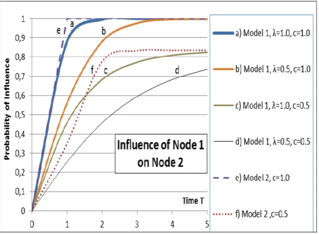
The saturation effect occurs sooner at T=1 in Model 2 as can be seen in Fig. 1 Curve e. From Equations (1–4) the proportion of spreading via Groups 1–4 could be calculated, but the probability of overall spreading from Node 1 to Node 2 must be calculated from Equation (5). In both models the probability of spreading approaches 1.0 when T approaches infinity.

In empirical social networks, nodes may be less than 100 % willing to change their opinions or to mediate the influence. Weighting factors less than 1.0 slow down the spreading process and the limiting values of probabilities for high values of T are less than 1.0. In Figure 2 the Curves c and d show the spreading, when the nodes have only 50 % probability to spread influence in Model 1 for the two values of the intensity parameter λ=1.0, 0.5. Both of these curves saturate at the value of 0.84 at high values of T. Curve f shows the effect of weighting factor c=0.5 in Model 2. The final state is not dependent on the temporal spreading model; the topology of the network and the weighting factors determine the equilibrium state of the nodes. However, during the spreading phase the probabilities of spreading increase with individual rates depending on the topology of the network, the weighting factors and the temporal spreading model. In Figure 2 the spreading is investigated only in one particular case, from Node 1 to Node 2.

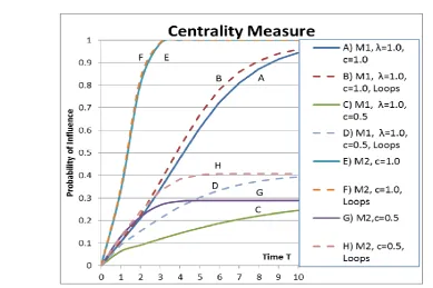
Figure 3 shows examples of numerical results calculated from Equation (8) in the two temporal spreading models for weighting factors c=1.0 and c=0.5. Curves A, B, C, and D show the probabilities of spreading in Model 1 with the intensity parameter λ=1.0 in Equation (12). Curves E, F, G, and H show the results from Model 2. Curves B, D, F, and H show the effect of loops on paths between source nodes and target nodes. In loops, the same nodes are allowed repeatedly. In the calculations, the shortest possible loops between two nodes are not allowed (e.g. 1-2-1-2 and 1-2-1-4). This is a practical choice in this paper; technically loops between two nodes may be possible in some applications.

The effect of weighting factors is important. The spreading is significantly slower with the weighting factor c=0.5 of curves C (Model 1) and G (Model 2) when compared with the corresponding curves A and E with c=1.0. The effect of loops is more prominent with c=0.5 than with c=1.0. Loops have a major effect when the spreading is slow and they have a negligible effect when the spreading is fast. The interpretation is that loops have no time to have major effects, if nodes are very active to spread influence in the network. At high values of time T curves C and G (D and H) approach a common limiting value, which is not dependent on the temporal spreading model.

Fig. 2: The spreading from Node 1 to Node 2 in the network structure of Fig. 1. Curves show the results from Models 1 and 2. The effect of intensity parameter λ in Model 1 and the effect of the weighting factor c in both

Fig. 3: Examples of numerical results from Equation (8) in the two temporal spreading models (M1 and M2) with weighting factors c=0.5, 1.0 with λ=1.0 (M1). The effect of allowing loops on paths is shown with dotted

curves B, D, F, and H.

V.

In Sections 5 and 6 the modelling method is illustrated with the help of the artificial network of Fig. 1. All the connections between nodes are assumed to be bidirectional. In Section 7 a real-world network will be investigated and centrality measures for the network calculated.

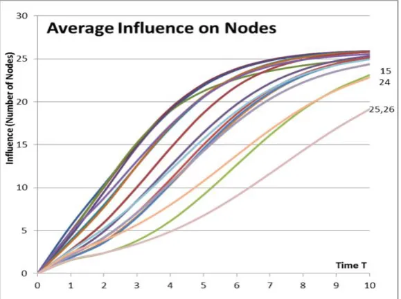
One node in the network is the source of spreading and other nodes are targets. In Figure 4 the probability of spreading from all the other nodes to Nodes 1–26 are shown as a function of time. The first temporal spreading model, Model 1, λ=1.0 and weighting factor c=1.0 are used. The convention of the value of probability 1.0 for the influence of Node 1 on itself is used in this paper (the other choice would be 0.0).

Some conclusions can be made from Fig. 4. The spreading is fast to nodes near the source node and slow to nodes far away. Consider the situation during the spreading phase when T<6. The spreading is slowest to Nodes {26, 25}, 24, 15, {17, 18, 19, 20, 21, 22, 23} in this order. The spreading is the same for nodes in curly brackets because of symmetry in the network topology. The equilibrium value is 26 with high values of time T because finally the spreading has reached all the nodes in the network.

The summation in Equation (8) is over target nodes of the network. Results in Fig. 4 are from Equation (9) where the summation is over source nodes of the network. Equations (8) and (9) have a natural interpretation: nodes in a social network have strong or small influence on other nodes (interpretation of Equation (8)) and, at the same time, nodes can be influenced by other nodes of the network strongly or weakly (interpretation of Equation (9)). Usually these values are not equal. This phenomenon may be enhanced in networks with unidirectional connections or weighted connections between nodes. In Figures 3–6 the corresponding Equation (8) or (9) is indicated to emphasize the case. The last column in Table 1 shows the spreading measure of the network from Equation (10) where the summation is over both indexes – source and target nodes.

It is possible that Pi,• in Equation (8) is high and P•,i in Equation (9) is zero. In this case, Node i has a

major influence on others but the other nodes don’t have any influence on Node i. In real life, dictators or very strong personalities may look like these. However, in many other cases the values of Pi,• and P•,i are highly

correlated. If there is a task of selecting a group of persons from a social network, these two quantities can be used in parallel for finding desired characters of individual persons and their composition as group members.

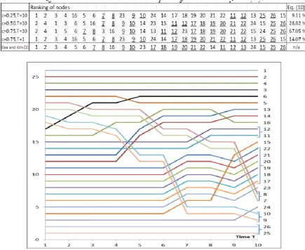
similar results with high weighting factors c=0.75 at low values time. In Table 1 this can be seen very clearly because the order of nodes’ influence is exactly the same (lines c=0.25, T=10 and c=0.75, T=1).

Results for c=0.5 and c=0.75 at time T=10 correspond saturated states when nodes are 50 % and 75 % active. Nodes 2, 4, 1, and 3 or 5 are most influential in this order. The rankings are different when compared with less active nodes (or early phases of the spreading process). When c=0.25 the rankings are 1, 2, 3, and 4. Node 16 is in a special position in the network of Fig. 1. Its influence is significantly less important when nodes are very active when c>0.5. In other words, the nodes having neighbouring nodes that are more connected with each other, like Nodes 2 and 4, get additional advantage. The relative ranking of Node 3 goes down for high weighting factors like the ranking position of Node 16.

In Table 1, the ranking results from [2] are also shown. They resemble the results for high activity nodes at high time T (c=0.75, T=10). There are some differences. Nodes 1 and 3 have higher rankings and Nodes 2 and 4 have lower rankings in [2], for example. On the other hand, if we compare the results for low activity nodes (c=0.25, T=10) the ranking is exactly the same for Nodes 1, 2, 3, and 4. Now the ranking of Node 16 is very different. In [2] the ranking is 9 and in our model the ranking is 5. Nodes 23 and 24 are peripheral nodes in the network and their ranking is also lower in [2].This difference can be a consequence of different dealing with network topologies like the structures around Nodes 1 and 16. Lawyer’s [34] work indicates that centrality measures can underestimate the spreading power of structurally peripheral nodes. Here, Node 16 has a high degree but in [2] another centrality measure called coreness centrality has been used. Another reason can be the lack of weighting factors as we have seen that in network spreading models the activity of nodes is a fundamental aspect to be considered. The equilibrium state at high values of T can be very different for low activity nodes than for high activity nodes. This is true also for the development phases during the spreading process.

We present an alternative way to illustrate the ranking of nodes. In Figure 6 the effect of Node 1 on other nodes is investigated in a detailed way (As said earlier, we use the numerical influence value 1.0 for the source node, Node 1). One important effect of network topology is that spreading is faster to nodes with several alternative paths to a target node. We take a look at low values of time T in Fig. 6. Spreading to Nodes 2, 4 and 3 is fast (in this order) compared to 5, {7, 8}, {9, 10}. Node 5 is reached faster than Nodes {7, 8} because there are more alternative paths to Node 5. Nodes {9, 10} have only one path from Node 1. When 6<T<10 most of the nodes are almost saturated and changes in ranking in this phase is not very important because the numerical values of the spreading measure are almost equal. At this phase, only Nodes 24, 25, and 26 have probability values significantly less than 1.0.

A more interesting feature is that the spreading from Node 1 to Node 6 grows faster when T>1 and gets higher than the spreading to Node {9, 10} when T>1.5 and to Nodes {7, 8} when T>2. Shortest paths from Node 1 to Node 6 are two connections compared to one connection for the other nodes but again more alternative paths are available. This example shows the dynamic behaviour of spreading. Ratios of probabilities are not constant as a function of time. In different phases of the spreading process spreading measures and rankings get different values as a result of the social network structure.

Fig. 5: Normalized values of the spreading measures for Nodes 1–26 (Equation (8)) in the first temporal spreading model with λ=1.0. The corresponding orders of nodes’ rankings are shown in Table 1.

Table 1: The rankings of Nodes 1–26 from Equation (8) with different activities of nodes c=0.25, 0.50, and c=0.75 at time T=10 (equilibrium). The third line shows the rankings at an early phase of the spreading process with T=1 and active nodes with c=0.75. The last line presents the ranking results from [2]. Nodes in symmetrical positions are indicated by underlining (or double underlining) where the spreading measures have the same values and rankings. The last column shows the network spreading measure from Equation (10).

VI.

SPREADING

The second aspect of influence spreading in social networks is the role of nodes as opinion mediators. In the literature, different measures for betweenness have been proposed for ranking and comparing the importance of nodes in networks [1], [6], [18], [47]. One possibility is to measure a node’s impact on the spreading by removing the node from the network. Consistently with Equations (7–9) Equation (13) can be defined as a betweenness measure. The normalization factor N2 has not been adjusted for the smaller network size. In Figs. 7–15 we will present quantities NBn(w,T) in units of number of nodes calculated from Equation

(13).





_{ }











 













_

_



n j i

j i

M

m

m j i

n

G

w

T

N

T

w

B

, 1

, 1

, ,

2

1

1

,

1

,

An alternative would be to measure the amount of influence mediated by the node to other nodes in the network. These measures are not equal because the topology is different when a node is removed from the network. The decisions which measure to use depend on the problem at hand. Removing a node implies that the objective is to eliminate the most influential node, and measuring the flow of influence via a node implies a more positive way of thinking to understand and possibly enhance influence spreading in the network. This enhancement could be achieved by two means. The node’s capability and activity can be enhanced or additional nodes in optimal positions can be implemented with the nodes of high betweenness.

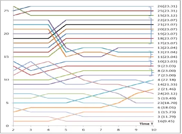
We consider removing one node from the network and investigate the consequences. In Figure 7 the ranking results from the first temporal spreading model (λ=1.0, c=1.0 are shown for the removed Nodes 1–26. In Figure 8 the same results are shown in units of number of nodes (sum over target nodes) as a function of time T. These two presentations illustrate two aspects of the spreading process: the changes in ranking of the nodes and the quantitative values of the spreading in the network. The curves show the network spreading measure from Equation (13). The most disruptive impact is caused by the removal of Node 16 when T>5. Node 16 cuts the connections between the two parts of the network and between the seven nodes directly connected to Node 16. Nodes 3 and 1 follow in this order.

Table 2: Model 1, Node 1 removed compared with the network of all the 26 nodes, λ=1.0, c=1.0, T=10 (Equation (8) in units of number of nodes).

It is notable that when T<5, removing Node 1 has the largest effect. This is a consequence of network topology and temporal spreading development in the network. When the spreading has just started from Node 1, it is more effective to spread influence via its neighbours compared to Node 16. However, if permanent or long lasting effects are pursued, Node 16 provides the strongest impact in the network. Removing Node 1 has only temporary effects because the spreading process proceeds in the network structure. The situation is different if the aim is to remove several nodes from the network. In this case, the optimal order of removing nodes starts from Node 1 when the spreading has not reached too far.

As an example we investigate the effects of removing Node 1. In Table 2 line 1 the average influence of source nodes (Nodes 2–26) on other nodes are shown in the network at time T=10 (the influence of Node 1 is 0.0). First of all, the maximum possible number of influenced nodes is 21 because Nodes {7, 8}, and {9, 10} are connected via Node 1 to the rest of the network. The influence of nodes {9, 10} is constant 1.0 and the influence of nodes {7, 8} approaches 2.0 as a function of time. Removing Node 1 from the network has changed the topology resulting in different spreading rates compared to the results of the original network of Fig. 1. The average value of the first line in Table 2 is 15.7 as can be seen in Fig. 8 at time T=10 corresponding the case where Node 1 is removed. For comparison, in Table 2 line 2, results at time T=10 when no nodes are removed are also shown.

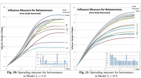
When T>5, the role of Node 3 is important because it cuts the connection between two parts of the network just like Node 16. The small bar charts in Figures 8–11 show the most important mediator nodes when T=10. At the final state the influence will not spread to all the nodes. The results from the second temporal spreading model are shown in Fig. 10. The choice of the temporal spreading model has only minor effects on the results. The ranking of nodes when paths with loops are allowed in the network are almost similar (not presented in this paper).

Next, we investigate removing one node from the network when the nodes are not 100 % active. The results (the first temporal spreading model, are shown in Fig. 9. The results show a significant difference when compared with Fig. 8. The order of nodes is 1, 3, and 16 instead of 16, 3, and 1. The network stays in its early development phase and because of the limited number of nodes in the network never reaches the later development phases identified in Fig. 8. Again the ranking results from the two temporal spreading models are almost similar. The results from the second temporal spreading model are shown in Fig. 11. The results with loops in the network show higher spreading rates indicating that the interactions are more important when the activity of nodes is not very high (not presented in this paper). The order of importance of nodes is almost the same as without loops.

Fig. 8: Spreading measure for betweenness in Model 1, λ=1.0, c=1.0.

Fig. 10: Spreading measure for betweenness in Model 2, c=1.0.

Fig. 11: Spreading measure for betwenness in Model 2, c=0.5.

VII.

In previous sections we have used an artificial network for illustration purposes. In this section a real-world network selected from public social network data bases is used to calculate centrality measures proposed in this paper. At the end of this section the betweenness measure of Equation (13) is discussed shortly. Bruce Kapferer has observed interactions in a tailor shop in Zambia [28]. The social network data represent two different types of interaction, sociational (friendship- and socioemotional) and instrumental (work- and assistance-related). Friendship data is bidirectional and work-related data is unidirectional. These networks have 316 and 109 links correspondingly. Data is available at two different times seven months apart but we use only the data from the beginning of the period.

The data enables us to demonstrate the method for weighted links in social networks. Link weights are taken as linear combinations of the binary information of the existing friendship- and work-related interactions. Schematically, the link weight used is 0.5(friendship) + 0.5(work-related). Other factors than 0.5 could be used depending on which kind of relations are more important in a particular application. The combined network for friendship and work-related network has 334 links. Interestingly, there are also some pure work-related links without a friendship- or socioemotional interaction. The selected network represents a typical, or somewhat larger, social network studied in the literature. Figure 12 shows the friendship network and Fig. 13 shows the combined network of friendship and work-related network. The social network has 39 nodes and some nodes, discussed in the text, are indicated in the figures.

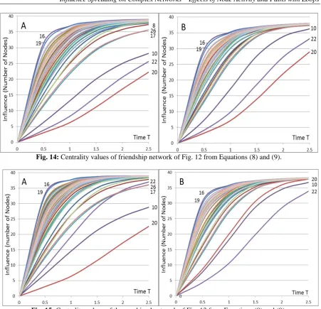
Figs. 14 and 15 show the values of the centrality measures as a function of time for the two networks of Figs. 12 and 13. Figures 14 A and 15 A show the centrality values of Equation (8) where the summation is over target nodes (outward view). Figures 14 B and 15 B show the centrality values of Equation (9) where the summation is over source nodes (inward view).

The model provides two different basic centrality measures. Figures 14 A and 14 B show that the two measures have different values even in a bidirectional network. This is a consequence of unsymmetrical network topology. The two centrality measures are even more different in Figs. 15 A and 15 B where a portion of the links between nodes are unidirectional and link weights are not equal.

The employees’ occupational categories and their prestige according to the survey among employees are known [28]. The head tailor is Node 19 and the cutter is Node 16. They have most interactions in both the friendship and work-related networks. As can be seen from Figs. 14 and 15 most of the workers don’t stand out from the results. Nodes 10, 20, and 22 have only one bidirectional friendship interaction with another node in the network. Nodes 8, 17, and 26 are connected with two bidirectional links. These are clearly seen in Fig. 14 A. In the network of Fig. 13 Node 22 has one bidirectional link, the same as in Fig. 12, and two outgoing work-related links. This can be seen in Fig. 15 A as a higher centrality value of Node 22.

Fig. 12: Sociational (friendship- and socioemotional) social network [28]. All the links are bidirectional.

Fig. 13: Combined network of sociational (friendship- and socioemotional) and instrumental (work- and assistance-related) social networks. Unidirectional links originate from the work-related data. For example there

Fig. 14: Centrality values of friendship network of Fig. 12 from Equations (8) and (9).

Fig. 15: Centrality values of the combined network of Fig. 13 from Equations (8) and (9).

One general feature of centrality values measuring outgoing interactions of Equation (8) when compared with incoming interactions of Equation (9) is seen in Figs. 14 B and 15 B. The curves show higher centrality values at higher values of time T for peripheral nodes like 10, 20, and 22 when compared with Figs. 14 A and 15 A. This is a consequence of the fact that, in spreading processes, initial phases at the beginning of processes is important for later development.

VIII.

Computational scalability of algorithms can be an issue for large networks. Contributions of all the different paths form a source node to target nodes are computed in the algorithm. As the number of potential routes increase with larger networks, the computing time increases accordingly. Initially, our goal has not been in putting efforts to developing an optimized algorithm. However, the algorithm has a feature of limiting the maximum path length in computations. In many cases, the most influential nodes in a network can be discovered with very short path lengths of 1–3 links. A general rule is difficult to give because dynamic behaviour and network topology can influence how long paths are needed. Obviously, if accurate numerical values of the measures are desired, in addition to just rankings, longer paths are necessary. Again, this has two viewpoints as computing numerical values for the most central nodes is faster compared to the peripheral nodes of a network. A numerical example illustrates this. Values of centrality measure from Equation (8) for Node 16 are 38.917, 38.998, and 39.000 with limiting path lengths of 4, 5, and 6 correspondingly. The values for Node 22 are 15.7, 22.6, and 25.8. For the central node, Node 16, numerical values are accurate with path length less than five but for the peripheral node, Node 22, path lengths longer than six are needed. In fact, this observation can be used to limit computing time when computing the centrality measure of Equation (8). This optimization occurs at the expense of accuracy of Equation (9) which, on the contrary, would require even longer path lengths.

Recently, a fast algorithm has been developed suitable for studying spreading processes like influence and opinion spreading. The algorithm is applicable for processes where nodes are allowed to appear several times in a path. However, then we must have a limit for path lengths or for the number of possible occurrences on the path. In this paper our focus is mainly on self-avoiding paths and small networks with loops allowed in paths. [27]

IX.

CONCLUSIONS

In this paper a new method is presented for calculating various spreading measures for general topological networks. The modelling is conducted in two phases: the temporal spreading model and the structure of the network with node and link characteristics can be taken as two distinct tasks. The method considers the structure of a network on a detailed level – individual nodes and connections can have their own characteristics, weighting factors or different temporal spreading distributions.

We have demonstrated the use of the method with the help of an artificial network. This network has been designed for modelling purposes [2]. The method is also used for a real-world social network [28]. The two different centrality measures proposed in this paper for two scenarios of the network are calculated and some results analysed, for instance the role peripheral nodes in the network. [32], [33]

The computing power is not an issue for small social networks studied, for example, in [1], [2]. In addition, the well-known rule of “six degrees” [48] allows us to set a higher limit to path lengths in computing approximate measures for large network structures. In summary, if only ranking nodes are of interest, the method proposed in this paper is scalable for different sizes of networks. If accurate numerical values for centrality or betweenness measures are of interest, the method is scalable for small social networks of tens of nodes. A real-world example investigated in this paper has 39 nodes and 334 links, i.e. the average degree of nodes is less than ten. In addition, the scalability of the algorithm is better for central nodes than for peripheral nodes in a network.

The method is capable of dealing with different network sizes and sub-network structures. Probability theory is used for combining the spreading via different paths of a network from a source node to a target node. The method of computing the exact contribution of all the different paths in a network with analytical formulas is one of the main results of this study. The method is demonstrated by computing spreading centrality and spreading betweenness measures.

We summarize some results of our study. The temporal spreading modelling has a substantial effect on the results, although the two alternative temporal models used in this paper provide almost the same results when intensity parameters of the spreading models are set appropriately. Typically, due to the network structure, the ranking of nodes changes during the spreading process as a function of time.

APPENDIX

In our work, two different models for the spreading as a function of time are used. The first model has the structure of Table A1 for path lengths L and time T. The values for L=1,…,4 and T=1,…,10 with the parameter value λ =0.5 are listed in the table. The second model has the structure of Table A2. With these parameter values the spreading is faster in the second model than in the first model.

Table A1. Probability PL,Tof the successful spreading as a function of time T for path lengths L in Model 1

(Poisson distribution) with the intensity parameter value of λ=0.5.

PL,T T=1 T=2 T=3 T=4 T=5 T=6 T=7 T=8 T=9 T=10 L=1 0.393 0.632 0.777 0.865 0.918 0.950 0.970 0.982 0.989 0.993

L=2 0.090 0.264 0.442 0.594 0.713 0.801 0.864 0.908 0.939 0.960

L=3 0.014 0.080 0.191 0.323 0.456 0.577 0.679 0.762 0.826 0.875

L=4 0.002 0.019 0.066 0.143 0.242 0.353 0.463 0.567 0.658 0.735

Table A2. Probability PL,T of the successful spreading as a function of time T for path lengths L in Model 2

(Uniform distribution).

PL,T T=1 T=2 T=3 T=4 T=5

L=1 1.000 1.000 1.000 1.000 1.000

L=2 0.500 1.000 1.000 1.000 1.000

L=3 0.167 0.792 1.000 1.000 1.000

L=4 0.042 0.501 0.957 1.000 1.000

L=5 0.008 0.235 0.816 0.997 1.000

L=6 0.001 0.085 0.567 0.967 1.000

L=7 0.000 0.025 0.309 0.859 0.998

L=8 0.000 0.006 0.134 0.648 0.980

L=9 0.000 0.001 0.049 0.396 0.903

L=10 0.000 0.000 0.015 0.197 0.733

REFERENCES

[1]. F. Agneessens, S. P. Borgatti, and M. G. Everett, ”Geodesic based centrality: Unifying the local and the global,” Social Networks vol. 49, pp. 12-26, 2017.

[2]. J. Bae and S. Kim, “Identifying and ranking influential spreaders in complex networks by neighborhood coreness,” Physica A vol. 395, pp. 549-559, 2014.

[3]. P. Basaras, D. Katsaros, and L. Tassiulas, “Detecting Influential Spreaders in Complex, Dynamic Networks,” Computer, vol. 46:04, pp. 24-29, 2013.

[4]. F. Bauer and J. T. Lizier, “Identifying influential spreaders and efficiently estimating infection numbers in epidemic models: a walk counting approach,” EPL (Europhysics Letters), vol. 99:6, 2012.

[5]. S. P. Borgatti, “Centrality and network flow,” Social Networks vol. 27, pp. 55-71, 2005.

[6]. S. P. Borgatti, “Identifying sets of key players in a social network,” Comput. Math. Organiz. Theor. vol. 12, pp. 21-34, 2006. [7]. S. P. Borgatti and M. Everett, ”A Graph-theoretic perspective on centrality,” Social Networks vol. 28, pp. 466-484, 2006.

[8]. D. Braha and Y. Bar-Yam, “From Centrality to Temporary Fame: Dynamic Centrality in Complex Networks,” Complexity, vol. 12, pp. 59–63, 2006.

[9]. D. Chena, L. Lüb, M. Shanga, Y. Zhanga, and T. Zhoua, ”Identifying influential nodes in complex networks,” Physica A vol. 391, pp. 1777–1787, 2012.

[10]. R. Cialdini, Influence: Science and Practice. Boston, MA: Pearson Education. ISBN 0-205-60999-6, 2009. [11]. M. DeGroot, “Reaching a Consensus,” J. Amer. Stat. Assoc., vol. 69, n. 345, pp. 118-121, 1974.

[12]. B. Doerr, M. Fouz, and T. Friedrich, “Why rumors spread so quickly in social networks,” Commun. ACM, vol. 55:6, pp. 70–75, 2012.

[13]. Y. Dua, C. Gaoa, and Y. Hub, S. Mahadevanc, Y. Denga, “A new method of identifying influential nodes in complex networks based on TOPSIS,” vol. 399, pp. 57–69, 2014.

[14]. M. Everett and S. P. Borgatti, ”Ego network betweenness,” Social Networks vol. 27, pp. 31-38, 2005.

[15]. M. Everett and S. P. Borgatti, ”Networks containing negative ties,” Social Networks vol. 38, pp. 111-120, 2014. [16]. N. E. Friedkin, “Norm formation in social influence networks,” Social Networks vol. 23, pp. 167–189, 2001.

[17]. N. E. Friedkin, “Social Influence Network Theory: Toward a Science of Strategic Modification of Interpersonal Influence Systems,” Dynamic Social Network Modelling and Analysis: Workshop, pp. 89-100, 2003.

[18]. L. C. Freeman, “Centrality in social networks: Conceptual clarification,” Social Networks, vol. 1 (3), pp. 215–239, 1979.

[19]. Y. Fua, C. Huang, and C. Suna, ”Using global diversity and local topology features to identify influential network spreaders,” vol. 433, pp. 344–355, 2015.

[20]. C. Gao, D. Weia, Y. Hub, S. Mahadevanc, and Y. Denga, “A modified evidential methodology of identifying influential nodes in weighted networks,” Physica A, vol. 392:21, pp. 5490–5500, 2013.

[21]. S. Gao, J. Maa, Z. Chena, G. Wang, and C. Xinga, “Ranking the spreading ability of nodes in complex networks based on local structure,” Physica A, vol. 403, pp. 130–147, 2014.

[22]. T. Gross and H. Sayama, Eds., Adaptive Networks: Theory, Models and Applications, Springer, 2009.

[23]. S. A. Hill and D. Braha, “Dynamic Model of Time-Dependent Complex Networks,” Physical Review E, vol. 82, 046105, 2010. [24]. P. Holme and J. Saramäki, Temporal Networks, Springer, 2013.

[25]. B. Houa, Y. Yaoa, and D. Liaob, “Identifying all-around nodes for spreading dynamics in complex networks,” Physica A, vol. 391:15, pp. 4012–4017, 2012.

18

[27]. M. Ijäs, J. Levijoki, and V. Kuikka, “Scalable Algorithm for Computing Influence Spreading Probabilities in Social Networks,” 5th European Conference on Social Media (ECSM 2018), Limerick Institute of Technology, Ireland, 2018.

[28]. B. Kapferer, Strategy and transaction in an African factory, Manchester: Manchester University Press, 1972.

[29]. H. Kelman, “Compliance, identification, and internalization: Three processes of attitude change,” Journal of Conflict Resolution vol. 2, pp. 51–60, 1958.

[30]. M. Kitsak, L. K. Gallos, S. Havlin, F. Liljeros, L. Muchnik, H. E.Stanley, and H. A. Makse, “Identification of influential spreaders in complex networks,” Nat. Phys. Vol. 6 (11), pp. 888–893, 2010.

[31]. K. Klemm, M. Á. Serrano, V. M. Eguiluz, and M. S. Miguel, “A measure of individual role in collective dynamics,” Sci Rep. vol. 2: p. 292, 2012.

[32]. V. Kuikka, “Influence Spreading Model Used to Community Detection in Social Networks,” in C. Cherifi, H. Cherifi, M. Karsai, M. Musolesi, Eds., Complex Networks & Their Applications VI. COMPLEX NETWORKS 2017. Studies in Computational Intelligence, vol. 689. Springer, Cham, 2018.

[33]. V. Kuikka, “Terrorist Network Analyzed with an Influence Spreading Model,” Complenet ’18, to be published in the conference proceedings in Springer's Complexity series, 2018.

[34]. G. Lawyer, “Understanding the influence of all nodes in a network,” Scientific Reports vol. 5, Article number: 8665, 2015. [35]. H. H. K. Lentz, T. Selhorst, and I. Sokolov, “Unfolding Accessibility Provides a Macroscopic Approach to Temporal Networks,”

Phys. Rev. Lett. Vol. 110, 2013.

[36]. Q. Li, T. Zhou, L. Lv, and D. Chen, “Identifying influential spreaders by weighted LeaderRank,” Physica A, vol. 404, pp. 47-55, 2014.

[37]. Z. Li, X. Tang, B. Chen, J. Yang, and P. Su, “Why continuous discussion can promote the consensus of opinions?” Computational Social Networks vol. 3:9, 2016.

[38]. J. Liu, Z. Ren, and Q. Guo, ”Ranking the spreading influence in complex networks,” Physica A vol. 392 pp. 4154–4159, 2013. [39]. J. C. Miller and I. Z. Kiss, ”Epidemic Spread in Networks: Existing Methods and Current Challenges,” Math. Model. Nat. Phenom.,

vol. (9)2, pp. 4-42, 2014.

[40]. M. E. J. Newman, “A measure of betweenness centrality based on random walks,” Social Networks vol. 27(1), pp. 39-54, 2003. [41]. M. Piraveenan, “Percolation Centrality: Quantifying Graph-Theoretic Impact of Nodes during Percolation in Networks,” PLOS

ONE, vol. 8 (1), 2013.

[42]. Y. Sun, L. Ma, A. Zeng, and W. Wang, “Spreading to localized targets in complex networks,” Scientific Reports vol. 6, Article number: 38865, 2016.

[43]. A. Zenga and C. Zhanga, “Ranking spreaders by decomposing complex networks,” Physics Letters A, vol. 377:14, pp. 1031–1035, 2013.

[44]. X. Zhanga, J. Zhub, Q. Wanga, and H. Zhaoa, “Identifying influential nodes in complex networks with community structure,” Knowledge-Based Systems, VOL. 42, PP. 74–84, 2013.

[45]. Z. Zhao, X. Wang, W. Zhang, and Z. Zhu, “A Community-Based Approach to Identifying Influential Spreaders,” Entropy, vol. 17, pp. 2228-2252, 2015.

[46]. D. Weia, X. Denga, X. Zhanga, Y. Denga, and S. Mahadevanc, ”Identifying influential nodes in weighted networks based on evidence theory,” Physica A, vol. 392:10, pp. 2564–2575, 2013.

[47]. W. Wang, “Modeling influence diffusion in networks for community detection, resilience analysis and viral marketing,” PhD thesis, University of Iowa, http://ir.uiowa.edu/etd/2165, 2016.

[48]. D. J. Watts, Six Degrees: The Science of a Connected Age, W. W. Norton & Company Ltd. London, 2004.