www.nonlin-processes-geophys.net/22/371/2015/ doi:10.5194/npg-22-371-2015
© Author(s) 2015. CC Attribution 3.0 License.
Improved singular spectrum analysis for time series
with missing data
Y. Shen1, F. Peng1,2, and B. Li1
1College of Surveying and Geo-informatics, Tongji University, Shanghai, China 2Center for Spatial Information Science and Sustainable Development, Shanghai, China Correspondence to: Y. Shen ([email protected])
Received: 12 October 2014 – Published in Nonlin. Processes Geophys. Discuss.: 21 December 2014 Revised: 15 May 2015 – Accepted: 20 May 2015 – Published: 10 July 2015
Abstract. Singular spectrum analysis (SSA) is a powerful technique for time series analysis. Based on the property that the original time series can be reproduced from its princi-pal components, this contribution develops an improved SSA (ISSA) for processing the incomplete time series and the modified SSA (SSAM) of Schoellhamer (2001) is its special case. The approach is evaluated with the synthetic and real incomplete time series data of suspended-sediment concen-tration from San Francisco Bay. The result from the synthetic time series with missing data shows that the relative errors of the principal components reconstructed by ISSA are much smaller than those reconstructed by SSAM. Moreover, when the percentage of the missing data over the whole time se-ries reaches 60 %, the improvements of relative errors are up to 19.64, 41.34, 23.27 and 50.30 % for the first four princi-pal components, respectively. Both the mean absolute error and mean root mean squared error of the reconstructed time series by ISSA are also smaller than those by SSAM. The re-spective improvements are 34.45 and 33.91 % when the miss-ing data accounts for 60 %. The results from real incomplete time series also show that the standard deviation (SD) derived by ISSA is 12.27 mg L−1, smaller than the 13.48 mg L−1 de-rived by SSAM.
1 Introduction
Singular spectrum analysis (SSA) introduced by Broomhead and King (1986) for studying dynamical systems is a pow-erful toolkit for extracting short, noisy and chaotic signals (Vautard et al., 1992). SSA first transfers a time series into a trajectory matrix, and carries out the principal component
analysis to pick out the dominant components of the trajec-tory matrix. Based on these dominant components, the time series is reconstructed. Therefore the reconstructed time se-ries improves the signal-to-noise ratio and reveals the charac-teristics of the original time series. SSA has been widely used in geosciences to analyse a variety of time series, such as the stream flow and sea-surface temperature (Robertson and Mechoso, 1998; Kondrashov and Ghil, 2006), the seismic to-mography (Oropeza and Sacchi, 2011) and the monthly grav-ity field (Zotova and Shum, 2010). Schoellhamer (2001) de-veloped a modified SSA for time series with missing data (SSAM), which was successfully applied to analyse the time series of suspended-sediment concentration (SSC) in San Francisco Bay (Schoellhamer, 2002). This SSAM approach does not need to fill missing data. Instead, it computes each principal component (PC) with observed data and a scale fac-tor related to the number of missing data. Shen et al. (2014) developed a new principal component analysis approach for extracting common mode errors from the time series with missing data of a regional station network. The other kind of SSA approach process the time series with missing data by filling the data gaps recursively or iteratively, such as the “Caterpillar” SSA method (Golyandina and Osipov, 2007), the imputation method (Rodrigues and Carvalho, 2013) or the iterative method (Kondrashov and Ghil, 2006).
eigenvec-tors and a scale factor to compensate for the missing value. Moreover, we do not need to fill in the missing data recur-sively and iteratively as in Golyandina and Osipov (2007). The rest of this paper is organized as follows: the improve-ment of SSA for time series with missing data follows in Sect. 2, synthetic and real numerical examples are presented in Sects. 3 and 4 respectively, and then conclusions are given in Sect. 5.
2 Improved singular spectrum analysis for time series with missing data
For a stationary time seriesxi (1≤i≤N), we can construct
anL×(N−L+1) trajectory matrix with a window sizeL. Its Toeplitz lagged correlation matrix C is formulated by
C=
c(0) c(1) · · · c(L−1) c(1) c(0) . .. ...
..
. ... . .. c(1) c(L−1) · · · c(0)
. (1)
Each elementc(j )is computed by
c(j )= 1 N−j
N−j
X
i=1
xixi+j j=0,1,2, . . ., L−1. (2)
For matrix C, we can compute its eigenvalues λk and the
corresponding eigenvectors vk in descending order of λk
(1≤k≤L). Then theith element of thekth principal com-ponent (PC)akis computed by
ak,i= L
X
j=1
xi+j−1vj,k 1≤i≤N−L+1, (3)
wherevj,kis thejth element ofvk. We compute thekth
re-constructed components (RCs) of the time series with the kth PC as (Vautard et al., 1992)
xik= 1 i i P
j=1
ak,i−j+1vj,k 1≤i≤L−1
1
L L P
j=1
ak,i−j+1vj,k L≤i≤N−L+1
1
N−i+1
L P
j=i−N+L
ak,i−j+1vj,k N−L+2≤i≤N.
(4)
Since λk, the variance of thekth RC, is sorted in
descend-ing order, the first several RCs contain most of the signals of the time series, while the remaining RCs contain mainly the noises of time series. Thus the original time series is recon-structed with the first several RCs.
The SSAM approach developed by Schoellhamer (2001) computes the elementsc(j )of the lagged correlation matrix by
c(j )= 1 Nj
X
i≤N−j
xixi+j j =0,1,2, . . ., L−1, (5)
where bothxiandxi+jmust be observed rather than missed,
andNj is the number of the products ofxi andxi+j within
the sample indexi≤N−j. Then we compute the eigenval-ues and eigenvectors from the lagged correlation matrix C. The PCs are also calculated with observed data:
ak,i= L Li
X
1≤j≤L
xi+j−1vj,k 1≤i≤N−L+1, (6)
whereLi is the number of observed data within the sample
index fromi toi+L−1. The reconstruction procedure of time series from PCs is the same as SSA. The scale factor L/Li is used to compensate for the missing value.
In order to derive the expression of computing PCs for the time series with missing data, Eq. (3) is reformulated as ak,i=
X
i+j−1∈Si
xi+j−1vj,k+
X
i+j−1∈Si
xi+j−1vj,k, (7)
where 1≤i≤N−L+1, andSi andSi are the index sets of
sampling data and missing data respectively within the in-teger interval [i,i+L−1], i.e.Si∩Si=0 andSi∪Si=[i, i+L−1]. If PCs are available, we can reproduce the miss-ing values. Therefore, the missmiss-ing values in Eq. (7) can be substituted with PCs as
xi+j−1= L
X
m=1
am,ivj,m. (8)
Substituting Eq. (8) into the second term of the right-hand side of Eq. (7) yields
1− X
i+j−1∈Si
v2j,k
ak,i−
X
i+j−1∈Si
L
X
m=1,m6=k
vj,mvj,kam,i
= X
i+j−1∈Si
xi+j−1vj,k. (9)
Collecting all equations of Eq. (9) fork=1, 2, . . . ,L, we have
Giξi=yi, (10)
where
Gi=
1− P
i+j−1∈Si
v2
j,1 − P
i+j−1∈Si
vj,1vj,2 · · · − P
i+j−1∈Si
vj,1vj,L
− P
i+j−1∈Si
vj,2vj,1 1− P
i+j−1∈Si
v2
j,2 · · · − P
i+j−1∈Si
vj,2vj,L
. . . . . . . . . . . . − P
i+j−1∈Si
vj,Lvj,1 − P
i+j−1∈Si
vj,Lvj,2 · · · 1− P
i+j−1∈Si
ξi=
a1,i a2,i .. . aL,i
,yi=
P
i+j−1∈Si
xi+j−1vj,1
P
i+j−1∈Si
xi+j−1vj,2
.. . P
i+j−1∈Si
xi+j−1vj,L
. (12)
Since Gi is a symmetric and rank-deficient matrix with the
number of rank deficiency equaling the number of miss-ing data within the interval [xi, xi+L−1], the PCs ak,i
(k=1, 2, . . . ,L) are solved with Eq. (10) based on the fol-lowing criterion (Shen et al. 2014):
min: ξiT3−1ξi, (13)
where3is diagonal matrix of eigenvaluesλk, which is the
covariance matrix of PCs. The solution of Eq. (10) is as fol-lows:
ξi=3GTi
GTi 3Gi
−
yi. (14)
The symbol “–” denotes the pseudo-inverse of a matrix. If the non-diagonal elements of Gi are all set to zero,
Eq. (14) can be further simplified as ak,i=
1
1− P
i+j−1∈Si
vj,k2 X
i+j−1∈Si
xi+j−1vj,k
1≤k≤L,1≤i≤N−L+1. (15) Supposing thatv1,k=v2,k= · · · =vL,k=1/
√
Lat the miss-ing data points, the solution of Eq. (15) will be reduced to Eq. (6). Therefore, the SSAM approach is a special case of our ISSA approach. The first several PCs contain most vari-ance; the elementxi+j−1can be approximately reproduced with the first several PCs in Eq. (8).
The main difference of our ISSA approach from the SSAM approach of Schoellhamer (2001) is in calculating the PCs. We produce the PCs from observed data with Eq. (14) ac-cording to the power spectrum (eigenvalues) and eigenvec-tors of the PCs, while Schoellhamer (2001) calculates the PCs from observed data with Eq. (6) only according to the eigenvectors and uses the scale factor L/Li to compensate
the missing value. We have pointed out that this scale factor can be derived from Eq. (15), which is the simplified version of our ISSA approach, by supposing the missing data points with the same eigenvector elements. Therefore the perfor-mance of our ISSA approach is better than SSAM of Schoell-hamer (2001). The only disadvantage of our method is that it will cost more computational effort.
3 Performance of ISSA with synthetic time series The same synthetic time series as in Schoellhamer (2001) are used to analyse the performance of ISSA compared to SSAM. The synthetic SSC time series is expressed as
0 100 200 300
0 100 200 300
SSC(mg/L)
OCT DEC FEB APR JUNE AUG
Figure 1. Periodic signalcs(t )(top panel) and Synthetic time series
(bottom panel).
c(t )=0.2R(t )cs(t )+cs(t ), (16) whereR(t )is a time series of Gaussian white noise with zero mean and unit standard deviation;cs(t )is the periodic signal expressed as
cs(t )=100−25 cosωst+25(1−cos 2ωst )sinωsnt
+25(1+0.25(1−cos 2ωst )sinωsnt )sinωat. (17) The periodic signal oscillates about the mean value 100 mg L−1 including the signals with seasonal fre-quencyωs=2π/365 day−1, spring/neap angular frequency ωsn=2π/14 day−1 and advection angular frequency ωa=2π/12.5/24 day−1. The 1 year of synthetic SSC time seriesc(t ), starting at 1 October with 15 min time step, is presented at the bottom of Fig. 1, the corresponding periodic signalcs(t )is shown at the top of Fig. 1.
Although the selection of window length is an important issue for SSA (Hassani et al., 2012; Hassani and Mehmoud-vand, 2013), this paper chooses the same window length (L=120) as that in Schoellhamer (2001) in order to com-pare the performance of the proposed method with that of Schoellhamer. Using the synthetic time series we compute the lagged correlation matrix and the variances of each mode. The first four modes contain the periodic components, which account for 72.3 % of the total variance; in particular, the first mode contains 50.2 % of the total variance. In order to eval-uate the accuracies of reconstructed PCs from the time series with different percentages of missing data, following the ap-proach of Shen et al. (2014), we compute the relative errors of the first four modes derived by ISSA and SSAM with the following expression:
p= 1 N
N
X
i=1 s
(ai−a0)T(ai−a0) aT0a0
×100 %, (18)
10 20 30 40 50 60 0
5 10 15
10 20 30 40 50 60 0
20 40
10 20 30 40 50 60 0
20 40 60
10 20 30 40 50 60 0
50 100
Percentage of Missing Data(%)
Relative Error(%)
(1) (2)
(4) (3)
Figure 2. Relative errors of first four PCs (ISSA: red line; SSAM:
black line).
1 10 20 30 40 50 3
4 5
1 10 20 30 40 50 3
4 5
1 10 20 30 40 50 2
5 8
1 10 20 30 40 50 2
5 8
1 10 20 30 40 50 2
8 14
Number of Experiments
Root Mean Squared Errors(mg/L)
1 10 20 30 40 50 2
8 14 (1)
(3) (4)
(5) (6)
(2)
Figure 3. RMSE of 50 experiments, (1)–(6) represent percentage of
missing data ranging from 10 to 60 % in 10 % increments.
from data missing time series, anda0denotes the PCs recon-structed from the time series without missing data. We design the experiment of missing data by randomly deleting the data from the synthetic time series. The percentage of deleted data is from 10 to 60 % with an increase of 10 % each time. Then, we reconstruct the first four PCs from the data-deleted syn-thetic time series using both SSAM and ISSA, and repeat the experiments 50 times. The relative errors of the first four PCs are presented in Fig. 2, from which we clearly see that the accuracies of reconstructed PCs by our ISSA are obviously higher than those by SSAM, especially for the second and fourth PCs. In the case of 60 % missing data, the accuracy improvements are up to 19.64, 41.34, 23.27 and 50.30 % for the first four PCs, respectively.
We reconstruct the time seriesc(t )ˆ using the first four PC modes and then evaluate the quality of reconstructed series by examining the error 1c(t )ˆ = ˆc(t )−cs(t ). For the cases whose missing data are between 10 to 50 % over the whole time series, the reconstructed component of the time series
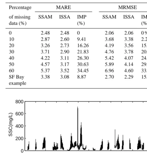
Table 1. Mean absolute reconstruction error and mean root mean
squared error of simulated time series with different percentage of missing data (mg L−1).
Percentage MARE MRMSE
of missing SSAM ISSA IMP SSAM ISSA IMP
data (%) (%) (%)
0 2.48 2.48 0 2.06 2.06 0 %
10 2.87 2.60 9.41 3.68 3.38 2.21
20 3.26 2.73 16.26 4.19 3.56 15.04
30 3.71 2.90 21.83 4.76 3.78 20.59
40 4.22 3.11 26.30 5.42 4.07 24.91
50 4.57 3.17 30.63 5.89 4.14 29.71
60 5.37 3.52 34.45 6.96 4.60 33.91
SF Bay 3.38 3.08 8.87 2.70 2.29 15.19
example
0 200 400 600 800
SSC(mg/L)
OCT DEC FEB APR JUNE AUG
Figure 4. Mid-depth SSC time series at San Mateo Bridge during
water year 1997.
is calculated only when the percentage of missing data in the window size is less than 50 %; while for the cases whose overall missing data already reach 60 %, 60 % missing data is allowed in the window size. In Fig. 3, we demonstrate the root mean squared errors (RMSEs) of each experiment of dif-ferent percentages of missing data. The RMSE is computed with1c(t )ˆ as
RMSE= v u u t
M
X
j=1 1cˆ2 t
j/M (19)
whereMis the number of data points involved in the exper-iment.
As can be seen from the Fig. 3, the RMSEs of ISSA are much smaller than those of SSAM for the same experiment scenarios. In Table 1, we present the mean absolute recon-struction error (MARE) and mean root mean squared error (MRMSE) of 50 experiments with different percentages of missing data.
im-Table 2. Maximum, minimum and mean absolute residuals of
SSAM and ISSA.
Residuals (mg L−1) SSAM ISSA
Maximum 145.05 126.61
Minimum −432.20 −227.70
Mean absolute residuals 8.19 8.00
SD 13.48 12.27
proved percentage (IMP) of ISSA with respect to SSAM is also listed in Table 1. As the amount of missing data in-creases, the IMPs of both MARE and MRMSE increase as well. Moreover, when the synthetic time series with the miss-ing data is same as the real SSC time series of Fig. 4, the IMPs of MARE and MRMSE are 8.87 and 15.19 %, respec-tively.
4 Performance of ISSA with real time series
The mid-depth SSC time series at San Mateo Bridge is pre-sented in Fig. 4, which contains about 61 % missing data. This time series was reported by Buchanan and Schoell-hamer (1999) and Buchanan and Ruhl (2000), and analysed by Schoellhamer (2001) using SSAM. We analyse this time series using our ISSA with the window size of 30 h (L=120) comparing with SSAM. The first 10 modes represent domi-nant periodic components as shown in Schoellhamer (2001) which contain 89.1 % of the total variance. Therefore, we re-construct the time series with the first 10 modes when the missing data in a window size is less than 50 %.
The residual time series, e.g. the differences of observed minus reconstructed data, are presented in Fig. 5. The max-imum, minimum and mean absolute residuals as well as the SD are presented in Table 2. It is clear that both max-imum and minmax-imum residuals are significantly reduced by using ISSA approach. The SD of our ISSA is reduced by 8.6 %. The squared correlation coefficients between the ob-servations and the reconstructed data from ISSA and SSAM are 0.9178 and 0.9046, respectively, which reflect that the re-constructed time series with our ISSA can indeed, to very large extent, specify the real time series.
5 Conclusions
We have developed the ISSA approach in this paper for pro-cessing the incomplete time series by using the principle that a time series can be reproduced using its principal com-ponents. We prove that the SSAM developed by Schoell-hamer (2001) is a special case of our ISSA. The perfor-mances of ISSA and SSAM are demonstrated with a syn-thetic time series, and the results show that the relative er-rors of the first four principal components by ISSA are
sig-−400 −200 0 200
−400 −200 0 200
SSC(mg/L)
OCT DEC FEB APR JUNE AUG
Figure 5. Residual series after removing reconstructed signals from
the first 10 modes (top panel: SSAM; bottom panel: ISSA).
nificantly smaller than those by SSAM. As the fraction of missing data increases, the improvement of the relative er-ror becomes greater. When the percentage of missing data reaches 60 %, the improvements of the first four principal components are up to 19.64, 41.34, 23.27 and 50.30 %, re-spectively. Moreover, when the missing data account for 60 %, the MARE and MRMSE derived by ISSA are 3.52 and 4.60 mg L−1, and by SSAM are 5.37 and 6.96 mg L−1. The corresponding improvements of ISSA with respect to SSAM are 34.45 and 33.91 %. When the missing data of synthetic time series is the same as the real SSC time series, the im-provements of MARE and MRMSE are 8.87 and 15.19 %, respectively. The SD derived from the real SSC time series at San Mateo Bridge by ISSA and SSAM are 12.27 and 13.48 mg L−1, and the squared correlation coefficients be-tween the observations and the reconstructed data from ISSA and SSAM are 0.9178 and 0.9046, respectively. Therefore, ISSA can indeed, to a great extent, retrieve the informative signals from the original incomplete time series.
The Supplement related to this article is available online at doi:10.5194/npg-22-371-2015-supplement.
Author contributions. Y. Shen proposed the improved singular
spectrum analysis and F. Peng wrote the FORTRAN program and performed the simulations. Y. Shen, F. Peng and B. Li prepared the paper.
Acknowledgements. This work is sponsored by the Natural Science
Foundation of China (Projects: 41274035, 41474017) and partly supported by State Key Laboratory of Geodesy and Earth’s Dynamics (SKLGED2013-3-2-Z).
Edited by: I. Zaliapin
References
Broomhead, D. S. and King, G. P.: Extracting qualitative dynamics from experimental data, Physica D, 20, 217–236, 1986. Buchanan, P. A. and Ruhl, C. A.: Summary of suspended-solids
concentration data, San Francisco Bay, California, water year 1998, Open File Report 99-189, US Geological Survey, San Francisco, 41 pp., 2000.
Buchanan, P. A. and Schoellhamer, D. H.: Summary of suspended solids concentration data, San Francisco Bay, California, water year 1997, Open File Report 00-88, US Geological Survey, San Francisco, 52 pp., 1999.
Golyandina, N. and Osipov, E.: The “Catterpillar”-SSA method for analysis of time series with missing data, J. Stat. Plan. Inf., 137, 2642–2653, 2007.
Hassani, H. and Mahmoudvand, R.: Multivariate singular spectrum analysis: a general view and new vector forecasting approach, Int. J. Energy Stat., 1, 55–83, 2013.
Hassani, H., Mahmoudvand, R., Zokaei, M., and Ghodsi, M.: On the Separability between signal and noise in singular spectrum analysis, Fluct. Noise Lett., 11, 1–11, 2012..
Kondrashov, D. and Ghil, M.: Spatio-temporal filling of missing points in geophysical data sets, Nonlin. Processes Geophys., 13, 151–159, doi:10.5194/npg-13-151-2006, 2006.
Oropeza, V. and Sacchi, M.: Simultaneous seismic data denoising and reconstruction via multichannel singular spectrum analysis, Geophysics, 76, 25–32, 2011.
Robertson, A. W. and Mechoso, C. R.: Interannual and decadal cy-cles in river flows of southeastern South America, J. Climate, 11, 2570–2581, 1998.
Rodrigues, P. C. and de Carvalho, M.: Spectral modeling of time series with missing data, Appl. Math. Model., 37, 4676–4684, doi:10.1016/j.apm.2012.09.040, 2013.
Schoellhamer, D. H.: Singular spectrum analysis for time series with missing data, Geophys. Res. Lett., 28, 3187–3190, 2001. Schoellhamer, D. H.: Variability of suspended-sediment
concentra-tion at tidal to annual time scales in San Francisco Bay, USA, Cont. Shelf Res., 22, 1857–1866, 2002.
Shen, Y., Li, W., Xu, G., and Li, B.: Spatiotemporal filtering of regional GNSS network’s position time series with missing data using principal component analysis, J. Geodesy, 88, 1–12, doi:10.1007/s00190-013-0663-y, 2014.
Vautard, R., Yiou, P., and Ghil, M.: Singular-spectrum analysis: A toolkit for short, noisy, chaotic signals, Physica D, 58, 95–126, 1992.