www.earth-syst-dynam.net/8/75/2017/ doi:10.5194/esd-8-75-2017
© Author(s) 2017. CC Attribution 3.0 License.
A network-based detection scheme for the jet stream
core
Sonja Molnos1,2, Tarek Mamdouh3, Stefan Petri1, Thomas Nocke1, Tino Weinkauf3,4, and Dim Coumou1,5
1Potsdam Institute for Climate Impact Research, Potsdam, Germany 2Department of Physics, University of Potsdam, Potsdam, Germany
3Department of Computer Graphics, Max Planck Institute for Informatics, Saarbrücken, Germany 4School of Computer Science and Communication, KTH Royal Institute of Technology, Stockholm, Sweden
5Institute for Environmental Studies (IVM), VU University Amsterdam, Amsterdam, the Netherlands
Correspondence to:Sonja Molnos ([email protected])
Received: 18 August 2016 – Discussion started: 29 August 2016
Revised: 11 December 2016 – Accepted: 12 January 2017 – Published: 10 February 2017
Abstract. The polar and subtropical jet streams are strong upper-level winds with a crucial influence on weather throughout the Northern Hemisphere midlatitudes. In particular, the polar jet is located between cold arctic air to the north and warmer subtropical air to the south. Strongly meandering states therefore often lead to extreme surface weather.
Some algorithms exist which can detect the 2-D (latitude and longitude) jets’ core around the hemisphere, but all of them use a minimal threshold to determine the subtropical and polar jet stream. This is particularly problematic for the polar jet stream, whose wind velocities can change rapidly from very weak to very high values and vice versa.
We develop a network-based scheme using Dijkstra’s shortest-path algorithm to detect the polar and sub-tropical jet stream core. This algorithm not only considers the commonly used wind strength for core detection but also takes wind direction and climatological latitudinal position into account. Furthermore, it distinguishes between polar and subtropical jet, and between separate and merged jet states.
The parameter values of the detection scheme are optimized using simulated annealing and a skill function that accounts for the zonal-mean jet stream position (Rikus, 2015). After the successful optimization process, we apply our scheme to reanalysis data covering 1979–2015 and calculate seasonal-mean probabilistic maps and trends in wind strength and position of jet streams.
We present longitudinally defined probability distributions of the positions for both jets for all on the Northern Hemisphere seasons. This shows that winter is characterized by two well-separated jets over Europe and Asia (ca. 20◦W to 140◦E). In contrast, summer normally has a single merged jet over the western hemisphere but can have both merged and separated jet states in the eastern hemisphere.
polar front and is driven by baroclinic eddies that evolve due to temperature gradients along the region of the polar front (Pena-Ortiz et al., 2013) and is therefore often referred to as an eddy-driven jet. Those transient eddies transport heat and vorticity and thereby accelerate the westerly winds (Woollings, 2010). The hemispheric north–south tempera-ture gradient is strongest in winter and weakest in summer, and this can explain variations in the jet stream strength and position between seasons. In summer, the winds are weaker and the jets move farther polewards, whereas in winter the winds are stronger and the jets move farther equatorwards as the cold front extends into subtropical regions (Ahrens, 2012).
Jet streams are thus sensible to changes in tempera-ture gradient and variability and hence also to climate change (Barnes and Polvani, 2013; Grise and Polvani, 2014; Solomon and Polvani, 2016). Large-scale undulations in the jets (Rossby waves) can sometimes become quasi-stationary (i.e., stagnant), which can lead to persistent weather condi-tions at the surface. Persistent weather can favor some types of extreme weather events (Coumou et al., 2014; Stadtherr et al., 2016). Petoukhov et al. (2013) proposed a mechanism that could provoke such weather extremes in the Northern Hemisphere midlatitudes. Quasi-stationary Rossby waves in summer are linked to persistent heat waves and severe floods (Kornhuber et al., 2016; Petoukhov et al., 2013, 2016). Like-wise in winter, strongly meandering jets, driven by either anomalous tropical (Palmer, 2014; Trenberth et al., 2014) or extratropical (Peings and Magnusdottir, 2014) sea-surface temperatures or stratospheric variability (Cohen et al., 2014; Kretschmer et al., 2016), can lead to midlatitude cold spells. Hence, jet streams play a key role in the general circula-tion and for generating midlatitude weather condicircula-tions and extremes.
Several schemes have been proposed to extract the jet stream positions from wind data, each one with advantages, but also limitations.
Rikus developed a detection method to analyze zonal-mean positions of the jet streams (Rikus, 2015) using the zonally averaged zonal wind in latitude–height space to iden-tify local maxima as cores of the jet streams. This method
Koch et al. (2006) classify so-called deep or shallow jet stream events. Their three-step algorithm first calculates the vertically averaged horizontal wind speed between two pres-sure levels (p1=100 hPa andp2=400 hPa) for each time in-stance and grid point. Next, a threshold of 30 m s−1is applied to detect a so-called jet event in a grid cell. Further analysis over vertical layers classifies events into deep or shallow jet stream events but it neither extracts the actual stream core, nor distinguishes between polar and subtropical jet streams (Koch et al., 2006).
Gallego et al. (2005) developed a scheme using a geostrophic streamline of maximum daily averaged velocity at 200 hPa to find the jet stream in the southern hemisphere. It uses wind velocitiy threshold of 30 m s−1and distinguishes between the subtropical and polar jet stream when the aver-age latitudinal difference is greater than 15◦. The threshold was set by manual optimization (Gallego et al., 2005). This approach might work reasonably for the southern hemisphere jets; a fixed threshold approach is particularly problematic for the Northern Hemisphere polar jet, which can change drastically in strength on weekly timescales.
The first 3-D method (longitude, latitude, height) devel-oped by Limbach at al. (2012), detects and tracks specific properties of atmospheric features as merging and splitting jet streams (via clustering of data points). Still, this method cannot distinguish between subtropical and polar jet streams and also requires the use of a wind velocity threshold (Lim-bach et al., 2012).
Another 3-D detection scheme was developed by Pena-Ortiz et al. (2013), which identifies local wind maxima in the zonal wind field by using a specified wind speed thresh-old. The algorithm distinguishes between the subtropical and polar jet stream via a specified threshold in latitude. A limita-tion of such an approach is that the values of such thresholds are not well defined. In particular the polar jet, which is our prime interest, can meander over large latitudinal ranges and experience strong variability in its strength (Pena-Ortiz et al., 2013).
cost function, defined by any combination of relevant vari-ables. We develop a 2-D detection scheme for both the PFJ and STJ core, and define our edge cost function using wind speed, wind direction and a latitudinal guidance parameter (which is not thresholded). This way, we are able to accu-rately differentiate between subtropical and polar jet.
In Sect. 2 we describe the data used in this algorithm. In Sect. 3 we explain the details of our detection scheme, parameter optimization process and its results. Afterwards (Sect. 4), we analyze jet stream positions from 1979 on-ward and calculate probabilistic maps for different seasons. In Sect. 5, we calculate trends in latitudinal position and wind strength for the STJ and the PFJ. We conclude with a sum-mary and a discussion in Sect. 6.
2 Data
In this study, we used ERA-Interim data (Dee et al., 2011) from the European Centre for Medium-Range Weather Forecasts (ECMWF). The ECMWF provides meridional and zonal wind velocity components with a 0.75 latitude– longitude grid resolution. We chose 11 vertical layers of the upper troposphere stretching from 500 to 150 mb and for four 6-hourly time steps per day (00:00, 06:00, 12:00, 18:00 UTC) for the years 1979–2014. From these data, we calculate 15-day running mean and vertically averaged (mass-weighted) wind velocity, which is used for all analysis in this paper.
In the following text, a “time period” denotes a 15-day mean centered on a given day.
3 Methods
Our jet stream core detection scheme is based on Dijkstra’s shortest-path algorithm, which is a widely used method for finding the shortest path from a source to a destination within an edge-weighted graph (Dijkstra, 1959). We assume that the jet stream core is a closed path along the hemisphere, with source (most westerly point) and destination (most easterly point) at the same location.
We use wind data on a two-dimensional grid of the North-ern Hemisphere, where each grid point is taken as a node in a network graph. Only geographically adjacent grid points (nodes) are connected via edges and thus no teleconnections are considered. The nodes within the most westerly column are copied after the end of the most easterly column to en-sure that that the path found with Dijkstra’s algorithm starts and ends at the same location. The path itself is not an injec-tive function of longitude meaning that the path can pass the same longitudinal coordinates multiple times.
To avoid noise and reduce computational costs only those grid points where the wind velocity is greater than 10 % of the maximum wind velocity for the considered time period are connected.
Figure 1.Definition of edge costs:(a)shows all nodes and edges as well as the wind velocities of the considered node (blue arrows) in the grid. The edge costs are computed from wind velocities (length of blue arrows,Xj), wind direction (angle between blue arrow and
black edge,Yj) and the latitudinal positionZj.(b) indicates the
third cost termZj of the STJ (blue) and PFJ (orange). The edge
cost is very low in the vicinity ofφclim=30◦N for the STJ and φclim=60◦N for the PFJ and very far away fromφclim.(c)shows
the STJ (black line) in the network graph over North and Central America for a certain time period.
In order to reduce computational costs, the spatial domain is reduced to the main region of interest, 0–75◦N, for the subtropical jet stream on the Northern Hemisphere. The spa-tial domain for the polar jet stream is 0–90◦N, since in some rare cases the polar jet stream could be occasionally close to the 30◦N limit.
We define an edge cost function, Cj, based upon wind
speed, wind direction and a latitudinal guidance function us-ing the climatological mean latitudinal position of each jet:
Cj=w1Xj+w2Yj+w3Zj
w1+w2+w3=1. (1)
The variablesXj ,Yj andZj, each normalized to the
inter-val [0, 1], are the three terms for computation of the cost at edgeej andw1,w2andw3are the weights that control the
contributions of the three cost terms. These weights are non-negative and their sum is equal to one.
The three terms and their respective factors are illustrated in Fig. 1a and b. Figure 1a shows all nodes and edges as well as the wind velocities of the considered node (blue arrows) in the grid. For each edge,ej, the cost is computed
depend-ing on the wind velocities (termXj, length of blue arrows)
and wind directions (termYj, angle between blue arrow and
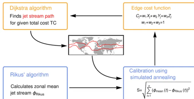
Figure 2.Calibration scheme. Before calculating the shortest path with Dijkstra’s algorithm, the cost of each edge has to be calculated according to the three termsXj,YjandZj. In order to find the correct weights of the terms, we calibrate them with simulated annealing and using Rikus’ algorithm to construct the skill function.
The first term, Xj, captures the magnitude of the wind
field at the nodes A and B. Jet streams are strong upper-level winds and hence the jet stream core should be where the wind strength is maximal:
Xj=1− q
u2A+vA2+
q u2B+vB2
2maxnk=1
q u2k+vk2
, (2)
where uA, uB, vA and vA are the zonal and meridional wind speeds at nodes A and B connected by edge j and
maxnk=1(
q
u2k+vk2) is the maximum wind speed found at the considered time period for any node k (see also Fig. 1a). The second term in Eq. (2) is thus always smaller than or equal to 1. We subtract this value from 1, and thus low values ofXjrefer to high wind speeds because Dijkstra’s algorithm
will minimize the edge cost of the path (i.e., find the shortest path).
The second termYj weights each edgeejaccording to the
angle between the normal vector of the edge and the wind direction:
Yj=
1− |VA| · ej
2 . (3)
Here|VA|is the normalized vector of the wind direction in node A and|ej|is the normalized vector of the edge direction
(see also Fig. 1a).
The third term, Zj, is used to differentiate between
po-lar and subtropical jet streams. Basically, it favors pathways that are close to the climatological mean latitude of polar and subtropical jets but still allows free movement within a lati-tudinal belt of roughly ±20 % of the climatological mean. Outside this latitudinal belt,Zrapidly grows according to
Zj=
φj−φclim 4
[max (φclim,90−φclim)]4. (4)
Here,φj andφclim are the latitude of the edge and of the climatological mean latitude, respectively.
The reason for taking the difference between the latitudes raised to the fourth power is to give flexibility to the detected path to move almost freely in the vicinity of the desired lat-itude, but a strongly increasing weight farther away. This is also illustrated in Fig. 1, where the conditionZj for the STJ
and PFJ is shown.
Naturally, there are other slightly different ways to define wind strength, wind direction and latitudinal dependence for the edges of the network. For example,Xj andYj could be
merged to a term which considers the wind projection along the edge unitary vector. In addition, it is possible to use a lower- or higher-ordered function for Eq. (4), e.g., a linear function or a function with the order of 8. However, a lower order means less free movement within the latitudinal belt centered aroundφclim. A higher order has negligible effects since Eq. (4) already gives values close to zero within the central latitudinal belt .
After calculating the edge cost for each edge according to Eq. (1), our algorithm returns from the set of all possible pathsPi with total edge costs of the path TCi the pathPmin
with minimal total edge cost TCmin:
TCMin=Min (TCi)=Min n X
j=0 Cj
!
, (5)
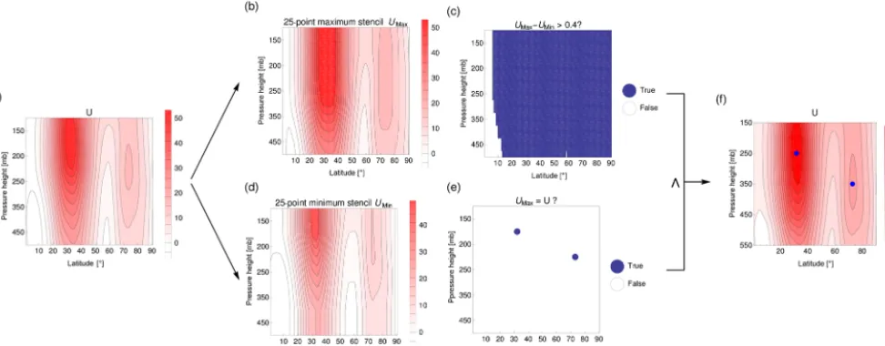
Figure 3.Rikus’ scheme. In(b)the 25-point maximum stencil (UMax) is calculated from(a)and in(d)the 25-point minimum stencil (UMin)
is calculated from(a). In(d)the conditionUMax(x,y)−UMin(x,y)>04 is examined and in(e)the conditionUMax(xy)=U(xy). Only
those points, where both conditions are fulfilled are zonal-mean jet stream cores, the blue points in (f) .
3.1 Calibration of weights
The optimal weightsw1,w2andw3and the climatological latitudeφclimare determined with a calibration scheme using simulated annealing and Rikus’ algorithm.
Rikus’ algorithm is a closed-contour object identification scheme (Rikus, 2015). It operates on a zonal-mean zonal wind and treats the two-dimensional (pressure height and lat-itude) zonal-mean U field for every time period as a single isolated image, using image coordinates defined by thexand y position.
Figure 3 shows the scheme of Rikus’ algorithm. First a local maximum or minimum filter is applied to the orig-inal zonal-mean U field. The maximum (minimum) filter is defined as a 25-point maximum stencil (25-point mini-mum stencil) applied to the totalU field. The stencil algo-rithm moves the maximum (minimum) value within a box of 5 points inx andy direction (resulting in a total of 25 grid points) to the central grid point of that box. The box with the central grid point (xy) moves over the totalU field starting at the upper left corner of the zonal-meanUfield and ending at the lower right corner.
This way, the fieldsUMinandUMaxare determined (Fig. 3b and c).
In a second step Rikus’ algorithm examines for each grid cell whether UMax(xy)−UMin(xy)>0.4 and whether UMax(x, y)=U(xy) (Fig. 4d and e). Only points where both conditions are fulfilled are zonal-mean jet stream cores (Fig. 3f, blue points).
We applied Rikus’ algorithm to the zonal-mean zonal wind field of each time period (i.e., 15-days running mean ERA-Interim data; Dee et al., 2011) to identify the zonal-mean jet stream latitude for all levels and latitudes in the domain
150–430 mb and 50–70◦N (15–50◦N) for the years 1979– 2014. We selected those days, where one polar and/or one jet stream within the above mentioned region was found. We used Rikus’ algorithm in a skill function to be minimized with simulated annealing to calibrate the weights of Eq. (1).
Simulated annealing (Kirkpatrick, 1984) is an optimiza-tion method that approximates the global minimum of a high-dimensional skill score function. We use the multi-run sim-ulation environment SimEnv (Flechsig et al., 2013) to cal-ibrate the weights w1 and w3 as well as φclim of Eqs. (1) and (4) for the PFJ and STJ separately. We define the skill function such that our results in the zonal mean match those of Rikus’ algorithm.
We expect the mean of all latitudinal positions calculated by our algorithm to be close to the zonal-mean jet position found by Rikus’ algorithm and thus define our zonal-mean skill function accordingly:
S=
tend
X
t=1 q
[φRikus(t)−φmean(t)]2, (6)
whereφmean(t) is the zonal-mean of all latitudes found by our algorithm andφRikus(t) is the zonal-mean latitude of the jet stream core determined by Rikus’ algorithm. We take the sum of the differences in latitude for all time periodstwhere Rikus’algorithm finds a jet core (tend is the number of such time periods). The scheme is illustrated in Fig. 2.
The reason for tuning our spatially resolved tool to a zonal-mean approach is that the characteristics of the jet stream such as the zonal-mean latitude position should be ultimately the same. The mean latitude detected by our algorithm should be very close to the maxima in zonal-mean zonal wind.
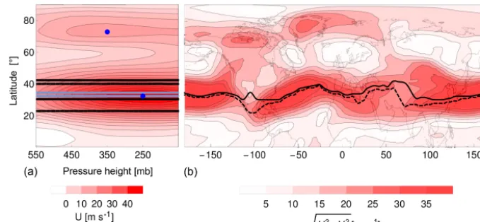
Figure 4.Panel(a): Zonal-mean latitude of the jet stream core calculated with Dijkstra’s algorithm using unoptimized weights (light-blue lines) and that computed with Rikus’ algorithm (blue circles). The black solid (dashed) lines are the borders of the PFJ (STJ) core latitude positions as calculated with Dijkstra’s algorithm. Panel(b): Polar (black) and subtropical (black dashed) jet stream cores are shown (15-day running mean around 13 January 2010).
Table 1.Start and optimized jet stream parameters used for the edge cost function.
Season Parameters Subtropical jet stream Polar jet stream start optimized start optimized
Cold
w1 0.49 0.044 0.49 0.044
w2 0.0015 – 0.0015 –
w3 0.5 0.95 0.5 0.95
φclim 30◦N 25.1◦N 60◦N 67.5◦N
Warm
w1 0.49 0.072 0.49 0.043
w2 0.0015 – 0.0015 –
w3 0.5 0.92 0.5 0.95
φclim 30◦N 29.8◦N 60◦N 69.1◦N
not affect the zonal-mean position used for tuning. For the manual tuning of w2, we tried different values for different time periods and found a value of 0.0015 to give the most desirable results. Since this weighting factor only affects lo-cal smoothing, its value does not affect the hemispheric path found.
As starting point for our automatic optimization scheme, the parameters (w1,w3andφclim) of the graph for Dijkstra’s algorithm were set to manually selected values as listed in Table 1. We chose the parametersw1andw3such that both parameters have approximately the same value. Forφclimwe chose the known climatology value for STJ and PFJ, respec-tively (Ahrens, 2012). Since the position of the jets changes depending on season, we allow our algorithm to alter this pa-rameter.
With the zonal-mean subtropical and polar jet stream lat-itudes found by Rikus’ algorithm we optimized the pa-rameters w1,w3andφclim for cold (November, December, January, February, March, April) and warm months (May, June, July, August, September, October). For computational reasons, we first optimize the STJ parameters using every
14th time period. This first step gives us proper starting con-ditions for the final optimization. Thus, in the final opti-mization we include all time periods and used as a starting point the optimized parameters found in the first step, which strongly speeds up convergence of the annealing method. For the polar jet stream, we used all jet stream cores found by Rikus’ algorithm.
3.2 Results of the optimization process
The results of our automatic optimization scheme are listed in Table 1. The jet stream guidance parameterw3needs to have a strong weight in order to separate the STJ and the PFJ. This large value ofw3is admissible, since Eq. (4), which de-scribes the latitudinal guidance, gives within the central lat-itudinal belt values close to zero. Hence the current choice still allows free movement of roughly±20 % of the climato-logical mean.
The climatological mean latitudeφclim shifts poleward in the warm season for both subtropical and polar jet, reflecting the seasonal cycle.
We would like to emphasize that all terms are important even thoughw3has the biggest value. If we consider onlyZj
and exclude all other terms, the jet stream core would be a straight line atφclim, since this would be the shortest path.
The zonal-mean latitudinal difference between Dijkstra (a longitudinally resolved latitude) and Rikus (a zonal-mean latitude) for the subtropical jet stream (<2◦) is always smaller than the difference for the polar jet stream (<5◦). This is indeed expected as the PFJ strongly meanders (Di Ca-pua and Coumou, 2016), whereas the STJ is strongly zonally oriented.
Figure 5.Fifteen-day running mean around 13 January 2010. Jet stream cores calculated with Dijkstra’s algorithm using optimized weights (compare with Fig. 2).
Figure 6.Fifteen-day running mean around 2 March 1979. The right panel shows three maxima (30, 50 and 75◦N); because of those three maxima, the mean jet stream core found with Dijkstra’s algorithm (light-blue line) does not match with the jet stream core found by Rikus’ algorithm (blue circle).
Table 1) are illustrated in Fig. 5. Here, the left panels show the zonal-mean latitude of the jet stream core calculated with Dijkstra’s algorithm (light-blue lines) and that computed by Rikus’ algorithm (blue circles). The black solid (dashed) lines are the borders of the PFJ (STJ) core latitudinal posi-tions as detected with Dijkstra’s algorithm around the hemi-sphere.
After tuning, the zonal-mean latitude of the polar jet stream core detected with Dijkstra’s algorithm is close to the latitude computed by Rikus’ algorithm (compare Fig. 5 with Fig. 4). Moreover, visual inspection of the right panel of Fig. 5 illustrates that our algorithm now correctly finds the polar jet around the hemisphere.
The mean latitude calculated with Dijkstra’s algorithm does not always match perfectly with the mean latitude com-puted by Rikus’ algorithm because the first is a 2-D algorithm in longitude and latitude and the latter is a 2-D algorithm in latitude and height. Rikus’ algorithm therefore does not cap-ture the undulations of the jet stream.
Often any such differences are related to the existence of not one but two zonal-mean PFJ maxima. For example, in Fig. 6 there exists a zonal-mean maximum at latitude ∼55◦N and another maximum at∼73◦N (left panel), but this is due to the undulation features of the jet stream pat-tern (right panel). Our algorithm resolves that undulation pattern, whereas Rikus’ only detects the stronger southerly maxima, since it searches in the range between 50 and 70◦N for the polar jet stream. For that reason, its mean latitude is in between the two maxima. Moreover, our approach is able to detect a high-over-low blocking situation for the PFJ, in contrast to, for example, Archer and Caldeira (2008) (see Sect. 1).
Figure 7.Fifteen-day running mean around 12 May 1979. The right panel shows only a maximum in the wind field in the region between 0 and 100◦E and around 70◦N latitude, which is the reason why the mean jet stream core found with Dijkstra’s algorithm (light-blue line) does not match with the jet stream core found by Rikus’ algorithm (blue circle) .
not the same. Figure 7 shows a situation where other paths for the STJ and the PFJ also could be considered with the jets split into two jet stream cores.
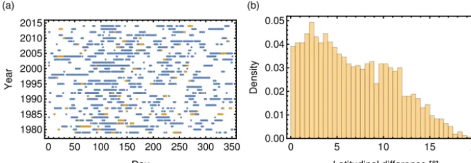
In Fig. 8 the differences between the zonal-mean polar jet stream cores calculated by Rikus’ algorithm and with Di-jkstra’s algorithm are shown in two different subplots. Fig-ure 8a shows a day–year plot depicting, in blue, days for which Rikus’ algorithm finds a polar jet stream in agree-ment with the range of jet stream core latitudes detected with Dijkstra’s algorithm. In yellow are those days where Rikus’ polar jet stream core position is not between the minimum and maximum latitude of the polar jet stream path detected with Dijkstra’s algorithm. These are 199 of 3122 data points which are equivalent to 6.4 %. Figure 8b shows the differ-ence between the mean latitude calculated by Rikus’ and the mean latitude calculated with Dijkstra’s algorithm. The mean of the difference is 5◦, but there are also some cases where the difference is much higher, up to 20◦. These differences are due to the undulations explained above.
The day–year plot of the subtropical jet stream in Fig. 9 shows that, for every single time period, Rikus’ latitude po-sition is within the range of latitudes found with Dijkstra’s al-gorithm. Figure 9b indicates the difference between the mean latitude calculated by Rikus’ and the mean latitude calculated with Dijkstra’s algorithm, which is very small. The mean is 2◦and the highest values are 6◦.
4 Jet stream probability analysis
In this section we present some results of the analysis of the jet stream paths that were detected by our algorithm.
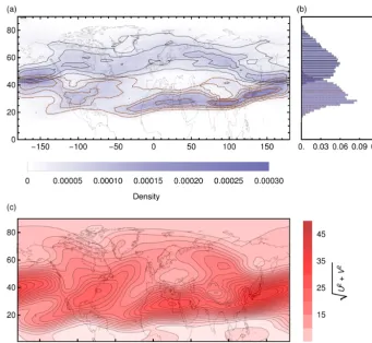
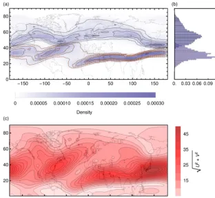
Figures 10–13 show probabilistic jet stream positions for different seasons with brown dashed contour lines represent-ing the subtropical jet and black solid contour lines repre-senting the polar jet.
The seasonal cycle of the STJ is clearly seen with winter latitudes between 20 and 40◦latitudes and summer latitudes further north. Moreover, in summer the probability that the jets merge in the western hemisphere is higher, whereas in winter the probability that they are clearly separated over al-most all longitudes is higher.
In addition, the probability frequency of the PFJ is much broader than the probability of the STJ and no clear latitudi-nal shift between seasons is observed. In particular, in sum-mer the PFJ distribution is smeared out (indicating large fluc-tuations in its position), whereas in winter it is more confined. This strong meandering of the eddy-driven PFJ is explain-able due to the nature of wave-mean flow feedbacks (Harnik et al., 2014). The PFJ cores always lie between 40–80◦N; only in longitudinal direction is there a seasonal dependence. Over Asia the probability of a high-latitude PFJ is larger in summer than in winter. Over Europe the probability of a low-latitude PFJ is higher in summer. This is also observable for eastern Pacific and North America , but less pronounced; in-stead there seem to be, in spring and summer, two preferable states: a merged jet state with a jet at ca. 50◦N and a second state with two jets at respectively ca. 50 and ca. 70◦N.
In general, the probability of PFJ at low latitude is small over the European sector compared to other regions and therefore double jet states occur in every season here. In North America such a clearly separated STJ and PFJ is only observed in winter.
Figure 8.(a)Day–year plot showing days used for tuning (blue) and those days where Rikus’ latitude position is not within the range of latitudes found with Dijkstra’s algorithm (199 of 3122 data points, 6.4 %)(b)Histogram of minimum latitudinal difference between the jet stream core found with Dijkstra’s algorithm and the mean latitude from Rikus’ algorithm, in degrees, for the polar jet stream.
Figure 9.(a)Day–year plot for the subtropical jet stream detection scheme (compare with Fig. 8).(b)Histogram of minimum latitudinal difference between the jet stream core found with Dijkstra’s algorithm and the mean latitude from Rikus’ algorithm, in degrees, for the subtropical jet stream.
PFJ are separated because the region of strongest baroclinic-ity is located relatively far poleward. In contrast, the region of strongest baroclinicity in the North Pacific is located near the latitude of maximum zonal wind, favoring a merged jet (Lee and Kim, 2003; Li and Wettstein, 2012). Such a merged jet stream is also called the eddy-thermally driven jet because of the two different genesis mechanisms. In special cases, there is the possibility that this eddy-thermally driven jet stream also appears over the North Atlantic (Harnik et al., 2014). This happens if the tropical forcing strengthens or the mid-latitude baroclinicity weakens.
In addition, Fig. 10–13b give probabilities of the zonal-mean latitude of both jets, showing enhanced variability of the PFJ compared to the STJ. The range of overlapping lati-tudes between STJ and PFJ is larger in summer than in winter because of the poleward shift of the STJ. The latitudinal vari-ability in STJ is lower in summer and winter than in spring and autumn, whereas the variability in the PFJ is similar be-tween seasons. However, the location of the maximum in the PFJ histogram changes per season: in winter, the maximum is at ca. 55◦N, whereas in summer there are two maxima at 50 and at 70◦N. These two maxima probably reflect the different behaviour in western and eastern hemisphere in the
PFJ. In spring, there is no clear maximum visible (between 40–60◦N), and in autumn it is again close to 55◦N.
To quantify those merged and separated states further, one could use the latitudinal difference between STJ and PFJ, for all longitudes, and this way create the probability density dis-tributions of merged and separated jets. The presented results (Figs. 10–13) might in principle also be the result of clearly separated jets which displace latitudinally over time to create the overlapping probability density.
For verification, we compare the probabilistic jet fields with seasonal climatological wind fields (panels c). In gen-eral, all probability density functions (PDFs) of the jet stream cores in their respective seasons coincide well with the wind fields. In summer, the wind field magnitude is very low and more homogeneously spread over the hemisphere. In sum-mer the jet stream cores are farther north than in winter due to the weaker temperature gradient in summer. In general, the gradient of the wind velocities, as well as the strength of the velocities, in summer is weaker than in winter.
5 Global trends
de-Figure 10.Probability analysis for spring months (MAM): Panel(a)and(b)show the spring probability density plot and a histogram of the jet stream occurrences (1979–2014). The brown dashed contour lines represent the subtropical jet stream, whereas the black solid contour lines represent the polar jet stream. Panel(c)depicts the climatological annual wind field (averaged over 1979–2014).
rived from our Dijkstra jet detection scheme. Table 2 sum-marizes the results giving linear trends in mean jet stream latitude and mean wind velocity with bold values indicating statistical significance (p <0.05).
In order to compare our results with literature results, we calculated mean jet stream latitude and mean wind velocity trends, which are shown in Table 2. Bold values indicate sta-tistical significance (p <0.05). We used Monte Carlo analy-sis with 10 000 surrogate time series of shuffled data to deter-mine significance (Di Capua and Coumou, 2016; Pollard and Lakhani, 1987; Schreiber and Schmitz, 2000). To account for the fact that running means present not data that is truly in-dependent data, we shuffle blocks of 15 days in this method. In general, we observe a northward trend for the STJ (ex-cept for SON) which is significant for winter and annual time series.T latitudinal position of the PFJ shows more mixed behavior with different signs for different seasons. A pro-nounced and significant equatorward trend is detected for the PFJ in winter. Wind velocities have generally weakened for both STJ and PFJ, something which is significant for sum-mer, in agreement with Coumou et al. (2015) and Lehmann and Coumou (2015).
Table 2.Slope parameter for the latitude and velocity trends of the jet stream cores. Bold values indicate statistical significance (p <0.05) using Monte Carlo analysis with 10 000 surrogate time series of shuffled data.
Season Subtropical jet stream Polar jet stream Latitude Velocity Latitude Velocity
◦decade−1 m s−1 ◦decade−1 m s−1
decade−1 decade−1
DJF 0.282 −0.021 −0.670 0.061
MAM 0.244 −0.454 0.004 −0.143
JJA 0.139 −0.259 −0.189 −0.147
SON −0.183 −0.263 0.049 −0.157
Annual 0.178 −0.321 −0.198 −0.085
Figure 11.Probability analysis for summer months (JJA; compare with Fig. 10).
Figure 13.Probability analysis for winter months (DJF; compare with Fig. 10).
30–60◦. Since STJ winds are in general stronger, we as-sume that, at least for spring, summer and autumn, their re-ported trends reflect trends of the STJ. Similarly, Archer and Caldeira (2008) considered only trends in Northern Hemi-sphere jet stream between 15–70◦N, where we again expect that this mostly reflects the behavior of the STJ. Rikus (2015) calculated trends for one northern jet stream core within 20– 54◦N, so we can assume that the trend most probably de-scribes the trend of the STJ. The findings of those studies can thus be best compared to our STJ findings. The annual pole-ward trend in latitudinal position of the STJ, detected with our method, is consistent with the results of Rikus (2015) and Archer and Caldeira (2008). Also, the latitudinal trend in summer calculated by our method has the same sign and order of magnitude as in Rikus and Pena-Ortiz et al., but the trend in winter is greater in our and Rikus’ method com-pared to that of Pena-Ortiz et al. The trends for spring and autumn agree in sign with the analysis of Pena-Ortiz et al. using 20th century data, but they are weaker and even change sign for the NCEP/NCAR data set in autumn.
The wind velocity trends are positive in the publication of Pena-Ortiz et al., whereas we observed a negative trend like that of Rikus (2015) (except summer) and Archer and Caldeira (2008). With our more advanced approach which is able to differentiate between subtropical and polar jet, we detect stronger (and mostly significant) weakening compared to the other studies.
6 Summary and discussion
We have proposed a novel and objective method to detect the subtropical and polar jet stream cores which overcomes some limitations of previous studies. Our method uses a graphi-cal approach employing Dijkstra’s shortest path algorithm. With this method we are able to describe both spatially sep-arated and merged jet stream cores. If the subtropical and polar jets merge, the two detected jet stream core positions become very close to each other.
We used three terms to define the edge costs: wind mag-nitude, wind direction and a jet stream latitudinal guidance term.
Based on those three terms, the algorithm finds the jet stream core as a closed path. Parameters entering this detec-tion scheme were optimized using simulated annealing and comparing our spatially resolved scheme with a zonal-mean detection scheme to avoid unrealistic results. Here we discuss some possible improvements to our scheme.
Figure 14.Annual, DJF, and JJA: mean latitudinal trends and mean wind velocity trends of the STJ and PFJ cores.
In addition, the jet stream latitudinal guidance term, which is in our case a fourth-order function of latitude, could be a lower- or higher ordered function like a linear function or a function with the order of 8. A lower order means less free-dom for the path to move away from the climatological lat-itude, whereas a higher order has only little effect, since the cost of a fourth-order function is already small in the latitu-dinal belt.
As a result the latitudinal guidance term seemed the most important factor. This large value ofw3is admissible, since Eq. (4), which describes the latitudinal guidance, gives
val-ues close to zero within the central latitudinal belt. Hence the current choice still allows free movement of roughly±20 % of the climatological mean.
dimensions and apply it to the southern hemisphere. Param-eters for the third dimension could be optimized in a similar way as done for latitude, but using pressure heights.
In addition, to account for splitting of the STJ and PFJ, we plan to calculate not two but four (or even more) jet stream cores with different climatological mean latitudes,φclim. In cases where only one path exists, the found jet stream cores would be combined to one path, (based on their similarities to each other) and in other cases where two paths exist, they would split.
Furthermore, we intend to analyze the influence and im-pacts of the jet stream to extreme events using cluster anal-ysis. This way, we can examine the link of particular cluster patterns on extreme weather events and determine which jet stream patterns have a higher probability for extremes. In ad-dition, we plan to find possible drivers which lead to those jet stream patterns, using causal effect networks (Kretschmer et al., 2016).
Another possibility is to apply our method to model data such as CMIP5 in order to analyze whether models can re-produce the jet accurately.
7 Code and data availability
All input data were downloaded from public archives. Code and data are stored in Potsdam Institute for Climate Impact Research’s long-term archive and are made available to in-terested parties on request.
Team list. Sonja Molnos, Tarek Mamdouh, Stefan Petri, Thomas Nocke, Tino Weinkauf and Dim Coumou.
Author contributions. Sonja Molnos, Tarek Mamdouh, Tino Weinkauf and Dim Coumou developed the study conception. Tino Weinkauf, Tarek Mamdouh and Thomas Nocke developed the analysis method. Sonja Molnos, Tarek Mamdouh and Ste-fan Petri developed the model code and performed the simulations. Sonja Molnos and Dim Coumou analyzed and interpreted the data. Sonja Molnos prepared the paper with contributions from all co-authors.
Edited by: R. A. P. Perdigão
Reviewed by: L. Rikus, C. Pires, and one anonymous referee
References
Ahrens, C. D.: Meteorology Today: An introduction to weather, cli-mate, and the environment, Brooks/Cole, Belmont, USA, 2012. Archer, C. L. and Caldeira, K.: Historical trends in the jet streams,
Geophys. Res. Lett., 35, 1–6, doi:10.1029/2008GL033614, 2008. Barnes, E. A. and Polvani, L.: Response of the midlatitude jets, and of their variability, to increased greenhouse gases in the CMIP5 models, J. Climate, 26, 7117–7135, doi:10.1175/JCLI-D-12-00536.1, 2013.
Cohen, J., Screen, J. A., Furtado, J. C., Barlow, M., Whittle-ston, D., Coumou, D., Francis, J., Dethloff, K., Entekhabi, D., Overland, J., and Jones, J.: Recent Arctic amplification and extreme mid-latitude weather, Nat. Geosci., 7, 627–637, doi:10.1038/ngeo2234, 2014.
Coumou, D., Petoukhov, V., Rahmstorf, S., Petri, S., and Schellnhuber, H. J.: Quasi-resonant circulation regimes and hemispheric synchronization of extreme weather in bo-real summer, P. Natl. Acad. Sci. USA, 111, 12331–12336, doi:10.1073/pnas.1412797111, 2014.
Coumou, D., Lehmann, J., and Beckmann, J.: The weakening sum-mer circulation in the Northern Hemisphere mid-latitudes, Sci-ence, 348, 324–327, doi:10.1126/science.1261768, 2015. Dee, D. P., Uppala, S. M., Simmons, A. J., Berrisford, P., Poli,
P., Kobayashi, S., Andrae, U., Balmaseda, M. A., Balsamo, G., Bauer, P., Bechtold, P., Beljaars, A. C. M., van de Berg, L., Bid-lot, J., Bormann, N., Delsol, C., Dragani, R., Fuentes, M., Geer, A. J., Haimberger, L., Healy, S. B., Hersbach, H., Hólm, E. V., Isaksen, L., Kållberg, P., Köhler, M., Matricardi, M., Mcnally, A. P., Monge-Sanz, B. M., Morcrette, J. J., Park, B. K., Peubey, C., de Rosnay, P., Tavolato, C., Thépaut, J. N., and Vitart, F.: The ERA-Interim reanalysis: Configuration and performance of the data assimilation system, Q. J. Roy. Meteorol. Soc., 137, 553– 597, doi:10.1002/qj.828, 2011.
Di Capua, G. and Coumou, D.: Changes in meandering of the Northern Hemisphere circulation, Environ. Res. Lett., 11, 94028, doi:10.1088/1748-9326/11/9/094028, 2016.
Eichelberger, S. J. and Hartmann, D. L.: Zonal jet structure and the leading mode of variability, J. Climate, 20, 5149–5163, doi:10.1175/JCLI4279.1, 2007.
Flechsig, M., Böhm, U., Nocke, T., and Rachimow, C.: The Multi-Run Simulation Environment SimEnv, available at: https://www.pik-potsdam.de/research/ transdisciplinary-concepts-and-methods/tools/simenv/ (last access: 4 February 2017), 2013.
Gallego, D., Ribera, P., Garcia-Herrera, R., Hernandez, E., and Gi-meno, L.: A new look for the Southern Hemisphere jet stream, Clim. Dynam., 24, 607–621, doi:10.1007/s00382-005-0006-7, 2005.
Grise, K. M. and Polvani, L. M.: The response of midlatitude jets to increased CO2: Distinguishing the roles of sea surface
tempera-ture and direct radiative forcing, Geophys. Res. Lett., 41, 6863– 6871, doi:10.1002/2013GL058489, 2014.
Harnik, N., Galanti, E., Martius, O., and Adam, O.: The anomalous merging of the African and North Atlantic jet streams during the northern hemisphere Winter of 2010, J. Climate, 27, 7319–7334, doi:10.1175/JCLI-D-13-00531.1, 2014.
Harnik, N., Garfinkel, C. I., and Lachmy, O.: Dynamics and Pre-dictability of Large-Scale, High-Impact Weather and Climate Events, edited by: JianPing, L., Richard, S., Richard, G., and Volkert, H., Cambridge University Press, Cambridge, 2016. Kirkpatrick, S.: Optimization by simulated annealing: Quantitative
studies, J. Stat. Phys., 34, 975–986, doi:10.1007/BF01009452, 1984.
Koch, P., Wernli, H., and Davies, H. C.: An event-based jet-stream climatology and typology, Int. J. Climatol., 26, 283–301, doi:10.1002/joc.1255, 2006.
Kornhuber, K., Petoukhov, V., Petri, S., Rahmstorf, S., and Coumou, D.: Evidence for wave resonance as a key mechanism for gener-ating high-amplitude quasi-stationary waves in boreal summer, Clim. Dynam., doi:10.1007/s00382-016-3399-6, in press, 2016. Kretschmer, M., Coumou, D., Donges, J. F., and Runge, J.:
Us-ing Causal Effect Networks to analyze different Arctic drivers of mid-latitude winter circulation, J. Climate, 29, 4069–4081, doi:10.1175/JCLI-D-15-0654.1, 2016.
Lee, S. and Kim, H.: The Dynamical Relationship between Sub-tropical and Eddy-Driven Jets, J. Atmos. Sci., 60, 1490–1503, doi:10.1175/1520-0469(2003)060<1490:TDRBSA>2.0.CO;2, 2003.
Lehmann, J., and Coumou, D.: The influence of mid-latitude storm tracks on hot, cold, dry and wet extremes, Scient. Rep., 5, 17491, doi:10.1038/srep17491, 2015.
Li, C. and Wettstein, J. J.: Thermally driven and eddy-driven jet variability in reanalysis, J. Climate, 25, 1587–1596, doi:10.1175/JCLI-D-11-00145.1, 2012.
Limbach, S., Schömer, E., and Wernli, H.: Detection, tracking and event localization of jet stream features in 4-D atmospheric data, Geosci. Model Dev., 5, 457–470, doi:10.5194/gmd-5-457-2012, 2012.
Palmer, T.: Record-breaking winters and global climate change, Sci-ence, 344, 803–804, doi:10.1126/science.1255147, 2014. Peings, Y. and Magnusdottir, G.: Forcing of the wintertime
atmo-spheric circulation by the multidecadal fluctuations of the North Atlantic ocean, Environ. Res. Lett., 9, 34018, doi:10.1088/1748-9326/9/3/034018, 2014.
Pena-Ortiz, C., Gallego, D., Ribera, P., Ordonez, P., and Del Car-men Alvarez-Castro, M.: Observed trends in the global jet stream characteristics during the second half of the 20th century, J. Geo-phys. Res.-Atmos., 118, 2702–2713, doi:10.1002/jgrd.50305, 2013.
Petoukhov, V., Rahmstorf, S., Petri, S., and Schellnhuber, H. J.: Quasiresonant amplification of planetary waves and recent Northern Hemisphere weather extremes, P. Natl. Acad. Sci. USA., 110, 5336–5341, doi:10.1073/pnas.1222000110, 2013. Petoukhov, V., Petri, S., Rahmstorf, S., Coumou, D.,
Kornhu-ber, K., and SchellnhuKornhu-ber, H. J.: The role of quasi-resonant planetary wave dynamics in recent boreal spring-to-autumn extreme events, P. Natl. Acad. Sci. USA, 113, 6862–6867, doi:10.1073/pnas.1606300113, 2016.
Pollard, E. and Lakhani, K. H.: The Detection of Density-Dependence from a Series of Annual Censuses, Ecology, 68, 2046–2055, 1987.
Rikus, L.: A simple climatology of westerly jet streams in global reanalysis datasets part 1: mid latitude upper tropospheric jets, Clim. Dynam., doi:10.1007/s00382-015-2560-y, in press, 2015. Schreiber, T. and Schmitz, A.: Surrogate time series, Physica D:
Nonlinear Phenomena, 2000, 142, 346–382, doi:10.1016/S0167-2789(00)00043-9, 2000.
Solomon, A. and Polvani, L. M.: Highly Significant Responses to Anthropogenic Forcings of the Midlatitude Jet in the Southern Hemisphere, J. Climate, 29, 3463–3470, doi:10.1175/JCLI-D-16-0034.1, 2016.
Son, S.-W. and Lee, S.: The Response of Westerly Jets to Thermal Driving in a Primitive Equation Model, J. Atmos. Sci., 62, 3741– 3757, doi:10.1175/JAS3571.1, 2005.
Stadtherr, L., Coumou, D., Petoukhov, V., Petri, S., and Rahm-storf, S.: Record Balkan floods of 2014 linked to planetary wave resonance, Sci. Adv., 2, e1501428, doi:10.1126/sciadv.1501428, 2016.
Trenberth, K. E., Fasullo, J. T., Branstator, G., and Phillips, A. S.: Seasonal aspects of the recent pause in surface warming, Nat. Clim. Change, 4, 911–916, doi:10.1038/nclimate2341, 2014. Woollings, T.: Dynamical influences on European climate: an
un-certain future, Philos. T. A. Math. Phys. Eng. Sci., 368, 3733– 3756, doi:10.1098/rsta.2010.0040, 2010.