www.nonlin-processes-geophys.net/17/431/2010/ doi:10.5194/npg-17-431-2010
© Author(s) 2010. CC Attribution 3.0 License.
Nonlinear Processes
in Geophysics
Stochastic resonance: from climate to biology
R. Benzi
Dipartimento di Fisica and INFN, Universit`a di Roma “Tor Vergata”, Via della Ricerca Scientifica 1, 00133 Roma, Italy Invited contribution by R. Benzi, recipient of the EGU Lewis Fry Richardson Medal 2006
Received: 8 April 2010 – Revised: 19 July 2010 – Accepted: 31 July 2010 – Published: 10 September 2010
Abstract. In this lecture, I will review some basic aspects of the mechanism of stochastic resonance, first introduced as a possible mechanism to explain long term climatic variation. Since then, there have been many applications of stochastic resonance in physical and biological systems. I will show that in complex system, stochastic resonance can substantially change as a function of the “system complexity”. Also, I will briefly mention how to apply stochastic resonance for the case of Brownian motors.
1 Introduction
The first numerical simulation providing strong evidence of Stochastic Resonance was performed by Angelo Vulpiani and myself on a rather exciting night in February 1980. Together with Alfonso Sutera and Giorgio Parisi, we were trying, at that time, to understand whether a relatively small periodic forcing can be amplified by internal nonlinear stochastic dynamics, leading to a possible understanding of the 100 Ky cycle observed in climate records. The first version of our paper was not accepted for publication by Science and Journal of Atmospheric Science. Eventually the paper was published in Tellus in 1982 (Benzi et al., 1982) together with a similar paper by Catherine Nicolis (Nicolis, 1981, 1982) who, independently, was proposing the same mechanism for climatic change. Shortly after that February night in 1980, we were able to provide a quite general understanding of how the mechanism works and how to generalize it for chaotic systems. Both theory and generalization appeared as a letter in J. Phys A in 1981 Benzi et al. (1981), i.e. one year before the Tellus paper!
Correspondence to: R. Benzi ([email protected])
We were, and we still are, convinced that Stochastic Resonance is a rather new and conceptually important phenomenon in science. For almost a decade, only few colleagues were sharing with us the same feeling. Eventually, after the paper of Moss and Wiesenfeld (1995) and some new theoretical work (McNamara and Wiesenfeld, 1989) stochastic resonance became a fashionable and interesting research topic in many different scientific areas from Climate to Biology, see Bulsara et al. (1993) and Giammaitoni et al. (1996) for a review.
Resonance is a kind of magic word in physics and there it is not surprising that a new resonance mechanism can excite the scientific community. In our case, the name stochastic resonance was introduce because of a short discussion with John Imbrie in March 1980. Just a few days after our first numerical simulation, I participated in a climate meeting in Erice where I gave a short talk on our results. John Imbrie, one of the most famous scientist working on paleoclimate, asked whether what we found was somehow similar to a resonance and my answer was: “not exactly! It is a kind of stochastic resonance!”. This is how the name was introduced. In some sense, we can think of a “resonance” as follows. In the standard resonance mechanism, think for instance of a damped harmonic oscillator, the amplification of the external forcing can be related, mathematically, to a singularity in the complex plane of the Green function of the problem. The real part of the singularity is, of course, the resonance frequency. In chaotic or stochastic systems, there are singularities in the complex plane but on the imaginary axis. The mechanism of stochastic resonance provides a way to shift the singularity in the complex plane. This rather cumbersome view of stochastic resonance may not be entirely clear but it tries to justify why the word “resonance” can still be used besides any historical reason.
resonance is still an interesting subject to work on and in particular I will discuss some new findings in simple and complex systems. Finally, I will mention how mechanisms related to stochastic resonance are of interest in the wide research field of Brownian motors.
2 The mechanism of stochastic resonance in climate theory
Climate is one of the most complex system in Nature and it is a major scientific challenge to understand the basic mechanisms leading to climate changes. In the past, climate showed quite remarkable changes over all times scales. In particular, one of the most striking aspects of past climate changes is the so called 100 ky cycles observed in paleoclimatic records. The cycle itself is not at all periodic, showing sudden warming phases followed by gentle decreases of temperature. This behaviour is in phase with the so called Milankovitch cycle, i.e. to the change of global radiation of the Sun due to astronomical change in the Earth orbit. This is the only global (i.e. averaged) change experienced in the incoming radiation. Is that possible to relate the astronomical forcing to the observed climate change? This is the basic question which puzzles scientific research since many decades. A simple computation shows that it is not easy to guess the correct answer.
Let us consider the simplest possible climate model. We consider the averaged Earth temperature T as the basic variable we want to describe, the precise meaning of average is of marginal interest for the time being. We know how much radiation is incoming, let us sayRin. The outcoming
radiationRoutdepends on the earth’s temperatureT (infrared
emission) and reflection from the surface, which can be written as αRin. Denoting by CE the Earth’s thermal
capacity, we can write the energy balance model as: CE
dT
dt =Rin−Rout (1)
whereRout=αRin+EIandEIbeing the infrared emission.
What we might call Earth’s climate is just the stationary solution of Eq. (1). WhileRin is independent ofT, bothα
andEIshould be dependent on the Earth’s climate which, in
our simple case, is described by the averaged temperature T. In a first approximation, we can think that EI is
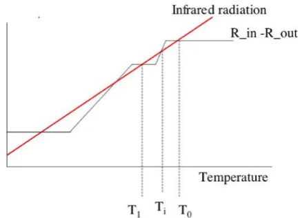
linearly dependent onT (a more complex behaviour does not substantially change the results). The so called albedoαis also aT-dependent quantity. More specifically, we expect αto be quite large for ice regions. An appropriate way to think of the functionα(T )is shown in Fig. 1. Following the cartoon shown in the same figure, it is clear that there exist more than one stationary solution of Eq. (1), corresponding to three different possible Earth climates. The coldest of the possible climates is referred to as “ice cover earth” climate, i.e. the case where almost all incoming radiation is reflected back to the space.
Fig. 1. The energy balance climate model. In the upper layer we show the basic variables of the model: the incoming radiationRin and the outcoming radiationRoutand the infrared emission. In the lower panel we show the albedo as a function of temperature Rin−Rout=(1−α(T ))Rin. The thick line represents the infrared emission.
Let us concentrate on the present (stable) climate. The orbital forcing, discovered by Milankovitch, is a small amplitude modulation ofRinin time, i.e.
Rin(t )=RSin+Acos(ωt ) (2)
Let us consider the effect of the Milankovitch forcing in Eq. (1). IfT is always quite close to the stationary (present) climateT0, we can estimateδT≡T−T0by:
dδT dt = −
1
τδT+Acos(ωt ), (3)
where 1/τ is the relaxation time of the present climate. More preciselyτ can be estimated by the equation:
1 τ = −
1 CE
[EI−(1−α(T ))Rin]
dT |T=T0
After an appropriate estimate of A, one can easily show using (3) that the effect of the orbital forcing on the present climate is of orderAτ∼0.5 K, much smaller than the 10 K observed in paleoclimatic records. Thus, it seems that orbital forcing can hardly explain the glacial/interglacial transition experienced by the Earth climate.
In order to make progress we need to supply our simple model by new features (for a detailed definition of the model see Benzi and Sutera, 1985). An important feature is to assume that there exist more than one stable climate state close to our present value T0. More precisely, we shall
about 10 K see Fig. 2. This is a rather ad hoc assumption which is, at any rate, consistent with observations of albedo. Still, this feature does not really change our conclusion since the orbital forcing is too small to provide a suitable mechanism to produce transitions betweenT0andT1.
The situation can improve dramatically if we consider the following three non trivial statements:
Many complex systems can be described by means of slow variables and fast variables, even if there is no explicit time scale separation between the two kind of variables. Fast variables may be considered as “noise” acting on the dynamics of slow variables.
For Earth climate, the averaged temperature in (1) should be considered as a slow variable with respect to the fast variables, due to weather variability.
When there exist multiple equilibria, the noise can introduce a long (random) time scale to switch from one equilibria to another.
The three statements are not trivial and should be explained carefully. For many decades, the splitting among slow and fast variables have been considered a well known feature of molecular motion. At the atomic scale, particles continuously experience short time interactions with other atoms while the hydrodynamic behavior (the slow variables) is described by a suitable space average over the molecular chaos. Looking at the fluctuating properties of a turbulent flow, there exists a well defined scale separation (both in time and in space) from molecular motion and hydrodynamic flow. Nevertheless, in a turbulent flow, even when disregarding any molecular motion, we can still distinguish large and small scale fluctuations. In this case, however, there is no spectral gap identifying any scale separation among scales. Therefore, one may be tempted to state that, in this case, the concepts of fast and slow variables are poorly defined. It turns out that such a statement is too limited. There exist experimental systems where the large scale motion can be thought as the slow variable superimposed to a noise (turbulent) small scale background acting on the system. Recently Benzi (2005), it has been shown that the above picture can explain qualitatively and quantitatively the numerical results observed in a simplified model of turbulence. Thus, in most complex systems the separation of large scale, slow variables and small scales, fast variables does correctly picture the dynamics in a self consistent way.
If we apply the above discussion to the Earth climate (second item), then on the time scale corresponding to the orbital forcing, the day-by-day weather fluctuations should be considered as noise (fast) variables acting on the climate system. This is not just a way of thinking. Disregarding the effect of noise is a major limitation for a correct description of the physical properties of climate. It took a long time,
Fig. 2. The albedo feedback for an energy balance model with three climate states nearT0. The model is conceptually similar to the one described in Fig. 1 with a change in the albedo.
and it is still ongoing, for the scientific community to accept that noise is not a measure of our “ignorance” but a physical feature of most complex systems.
The third item is more delicate and needs to be explained in details. Let us assume that our climate system (although the discussion is true for any system) shows two stable equilibria whose temperature difference is 21T. In this case, it is well known that the effect of the noise can induce transitions between the equilibria. The characteristic timeτL
for the transition can be estimated as: τL∼τexp
1T2/σ τ (4)
where, as in Eq. (3),τ is defined as the (fast) relaxation time over one of the stable equilibria andσ is the variance of the noise (weather fluctuations) acting on the system. Thus our year-by-year temperature is assumed to be decomposed into the climatic componentT and a fast noise component. In Eq. (4), τL should be considered an average time to switch
from one equilibria to another. In other words, the transition time between the two equilibria τeq is a random variable
with average valueτL. Actually, under some quite generic
conditions, we can predict the probability distribution ofτeq
which is P (τeq)=
exp −τeq/τL
τL
(5) Let me summarize the new feature we have introduced in the simple energy balance model (1). We have assumed a new form of the albedo which is providing three different climate states aroundT0, let us call themT1(stable),Ti (unstable)
andT0. The shape of the new albedo is shown in Fig. 2. We
assume thatT0−T1= 10 K andT0−Ti=Ti−T1. Next we
nearTi and simplify the equations by usingT=Ti+1T X
with1T=5◦K: dX
dt =X−X
3+√σ η(t ) (6)
whereη(t )is a Gaussian random variable with unit variance (hη(t )η(t0)i =δ(t−t0)) andσ is the noise strength. Notice that we have also rescaled the time unit.
In order to do some computation what we still need is the strength of the noise. We can obtain some information by the following argument. In our present climate (i.e.T0) we have
observational data which tell us about average temperature fluctuations. Also, we know from General Circulation Models, which is the time correlation for temperature fluctuations. Thus, we can estimate the strength of the noise by linearizing our climate model around T0 and using the
fluctuation-dissipation theorem, i.e. temperature variance = noise strength/(2 relaxation time). Once we know the noise strengthσwe can compute the average switching time from T0 toT1. It turns out that, by using (4) the average
transition time between the two stable states of our climate model is close to 50 000 years! This is a rather surprising and interesting result because it tells us that there exists a rather long time scale (50 000 years) introduced by the nonlinearity in the model and the noise, to be compared against the quite short time scale of the model, namely the deterministic relaxation time towards one of the two stable equilibria which is of the order of 10 years. However, this is not enough because the characteristic time of 50 000 years is a random time with an exponential probability distribution. Therefore nonlinearity and noise are not enough to get a periodic behavior of the temperature.
In order to get a periodic behavior, the idea is to introduce the Milankovitch effect in the system. After a simple computation one gets the following results:
dX
dt =X−X
3+Asin(ωt )+√σ η(t ) (7)
An appropriate rescaling in terms of physical quantities gives us the value ofA∼0.11 for the Milankovitch terms andω=
2π/105×1/10. Without the noise, the value ofX changes periodically in time with an amplitude order A. Going back to the temperature, this implies that, without noise, we have a periodic behavior of temperature with amplitude A1T ∼0.5 K. The situation changes completely when we consider the effect of the noise. A correct understanding of the noise effect can be achieved by considering the simplified equation:
dX
dt =X−X
3+A√σ η(t ) (8)
i.e. without any time dependency on the external forcing. It is crucial to remember that for any stochastic differential equation of the form:
dX dt = −
∂V ∂X+
√
σ η(t ) (9)
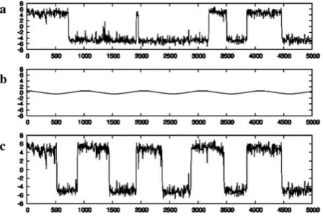
Fig. 3. Numerical simulation of Eq. (7) in three different cases. In the upper panel, we show the solution with the noise andA=0. In the middle panel we show the perturbing forcingAcos(2π ωt ) while in the lower panel we show the solution withA=0.1. The effect of the small periodic forcing is to synchronize the random switching from one climate states to the other, i.e. to get a stochastic resonance.
the “equilibria” probability distributionP (X)ofXis given by:
P (X)=ZNexp(−2V (X)/σ ) (10)
where ZN is a normalization factor. In our case V (X)= −1/2X2+1/4X4−AX(8) and we obtain from (10) P (X;A)=P (X;A=0)exp(2AX/σ ) (11) The probability distribution when A6=0 changes dramati-cally the probability distribution whenA=0. Even for small A the exponential factor 0exp(2A/σ ) can be rather large, i.e. order 30 in our case. The consequence of this simple calculation is that the probability to be nearX∼1 is 30 times larger than to be inX= −1. Now it is quite clear that if Ais slowly varying as cos(ωt )in time than the probability distribution is peaked periodically in ±1 with almost the same period of 2π/ω. This is the very essence of stochastic resonance.
One has to be a little careful in understanding the possible results of (7). As we said, the modulation ofAin time should be slow enough in order to get a stochastic resonance. We can be more quantitative using the following simple argument. Let us go back to Eq. (8). We can compute the probability distribution of the random time to go from+1 to−1 and we already know that the probability distribution is exponential. Letτ1(+1)be the average exit time, then the variance of the
random switching time is alsoτ1(+1). Finally we know how
to relateτ1(+1)toA, namely by using the expression:
τ1(+1)∼exp 2
σ(1V0+A)
(12) where in our case1V0≡1/4. Thus the requirement we need
is thatτ1(+1)2π/ωandτ1(−1)2π/ωwhereτ1(−1)is
the average exit time starting with the initial conditionX= −1. The two requirements imply
exp
21V0 σ
∼ 2π
ω , (13)
exp
2
σ(1V0−A)
2π
ω . (14)
The meaning of the above inequalities is represented in the cartoon of Fig. 4. The time increasesis clockwise, beginning with the left top panel. We start atX=1 and as time goes by, the system att=T /2 has a very high probability to jump toX= −1 if (14) is satisfied. Then at t=T we have the same effect for the transitionX= −1→X=1. The two conditions (13), (14) tell us that if the noise is too small then we will never see anything and, conversely, if the noise is too large transitions will happen regardless of the external periodic forcingA. Thus, there is a range ofσ ( the resonant range) where we obtain periodic transitions in phase with the external forcing.
One can highlight the resonance effect also by using another kind of variable. LetX(t )the solution of (7) and let us denote byFX(ν)its Fourier transform. Then|FX(ν)|2
represents the power spectrum ofX. We should expect that
|FX(ν=ω)|2is a function of the noise with some maximum
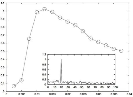
value for the “resonant noise”σR. This is indeed the case
as shown in Fig. 5, where|FX(ν=ω)|2is plotted againstσ,
while in the inset we show|FX(ν)|2forσ=σ|rmR.
Let us now returnto the climate. As we have seen, the effect of a small periodic forcing in our “simplified” climate model is to produce a periodic glaciation-interglaciation transition in phase with the Milankovitch forcing. However, the signal shown in Fig. 3 poorly compares against the observed behavior of the “proxy” earth temperature. The latter shows a kind of saw tooth behavior with strong asymmetries between cold and warm periods. Thus it seems that our theory cannot represent the real climate. Such a negative statement, however, is somehow misleading simply
Fig. 4. A cartoon to explain the mechanism of stochastic resonance. The period of the oscillation isT. At timet=0 the climate states has low probability to jump from+1 to−1. At timet=T /2 the situation is reversed: the probability no to jump is extremely small. At timet=T we start a new cycle.
because the model so far used, namely the energy balance model (6), includes only the simplest possible feedback due to radiation. More sophisticated effects, like the temperature-precipitation effect, can change the situation. Based on the above discussion we can make the following statement:
stochastic resonance is able to show that the external “weak” forcing due to Milankovitch cycle can be amplified by internal non linear dynamics of the climate;
climate dynamics shows a long time scale behavior due to non linear feedback;
noise can develop long time scale behavior if there exists multiple equilibria;
The most important feature coming out of our analysis is that it is crucial to understand the non linear interaction between fast a and slow time variables in climate models. Time scales of order 1000 years or more, do no rule out the importance of the dynamics of fast variables usually characterize atmospheric and/or oceanic circulations’. This, I think, is an important feature even in more sophisticated and/or realistic climate models.
Fig. 5. The figure shows the Fourier amplitude|FX(ν=ω)|2for
the solution of Eq. (7) for different values of the noise amplitudeσ. In the inset we show|FX(ν)|2forσ=σR, i.e. the optimal noise for which the Fourier amplitude atν=ωis maximum.
rather peculiar behavior calls for an explanation which, not surprisingly, can be given in terms of stochastic resonance. As we previously discussed for Eq. (7), the effect of the periodic forcing is to decrease or increase (depending on the timet) the probability of switching from a climate state to the other. With reference to Fig. 4, if at timet=T /2 the system does not switch, then it takes a full period T for the possibility to make a jump. This is certainly the case if the noise intensity is smaller thanσR. It follows that the
probability of the exit time is not peaked aroundT /2 but is quantized with maxima in(2n+1)T /2,n=1,2,.... To show that our analysis is correct, in Fig. 6 we plot the probability distribution of switching time forσ=0.8σR(symbols) and
for σ=σR (continuous lines). The quantization effect is
quite clear, as predicted by our simple analysis.
It appears that the observation of Alley et al. may be explained by the mechanism of stochastic resonance as it was pointed out by the these authors. Actually, a theoretical analysis of a simplified ocean/atmospheric model, due to Ganopolski and Rahmstorft (Ganopolski and Rahmstorf, 2002) shows that the effect of a periodic forcing in freshwater input over the North Atlantic Ocean combined with a suitable stochastic forcing, produces stochastic resonance in cold/warm climate changes as observed in real data. In the Ganopolski and Rahmstorft model, the two climate states, between which one has climate transitions, represent two different thermoahline circulation in the Norht Atlantic Ocean, which are responsible for sea ice growth and destruction.
It is unclear, at this stage, whether stochastic resonance is or is not the possible explanation of the Alley et al. data and more research is needed for a reasonable assessment. At any rate, it is important to remark that abrupt climate changes, such as those observed during the Milankovitch cycle or over
Fig. 6. Probability distribution of the random switching timeτ for two different noise amplitude obtained as the solution of Eq. (7). The amplitude and the period of the forcing is the same. Line refers toσR(see Fig. 5) while symbols refer toσ=0.8σR. In the inset we show the probability distribution of the random switching time in log-lin plot. It is evident that forσ smaller thanσRthe probability distribution ofτis “quantized” at integer values of(2n+1)T /2.
the last 100 000 years are hard to explain without the idea of transition between multiple equilibria triggered by noise, which is the basic feature of stochastic resonance (Sutera, 1981).
3 Stochastic resonance in complex systems
In the last ten to fifteen years the mechanism of stochastic resonance has been widely applied to a number of different physical and biological systems. Among them, the most striking applications concern neural systems pioneered, by Moss and collaborator (Moss and Wiesenfeld, 1995). In most cases, experimental results show a remarkable agreement with respect to the qualitative and quantitative picture represented in Fig. 6. Also, in many applications one does not know the “equation of motions” for the system and, actually, periodic perturbations leading to a stochastic resonance are used as a “measure” of non trivial cooperative phenomena in the system under study (this is certainly the case for most neurophysiological systems).
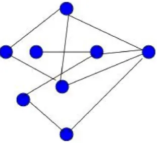
When dealing with complex systems, one can find non trivial behavior of the stochastic resonance. In this section we show that this is the case for a network system composed by some “node”ψi,i=1,...N, see Fig. 7.
Just to simplify the discussion, let us assume that the dynamics of each node is controlled by the same equation and that the connectivity of the system is described by the matrix Lij:
dψi
dt =mψi−gψ
3
i +Lijψj+
√
σ ηi (15)
that P
iLijψj≡0 which clearly can be done without lack
of generality, and finally, that P
iLi,jψiψj >0, i.e. the
connectivity matrix does not introduce any “instability” in the dynamics of the system. The noiseηi isδ-correlated in
time andhηiηji =δij.
The complexity of our problem, so to speak, is introduced by the matrix Lij. We want now to study the behavior of (15)
when an external periodic forcing is added to the system, i.e.
dψi
dt =mψi−gψ
3
i +Lijψj+
√
σ ηi+Aicos(2ωt ) (16)
In order to simplify our work, let us focus on the “average” variable8=N−1P
iψi. One should expect that for long
enough period T =2π/ω and a suitable noise σR(m,g) a
stochastic resonance can be observed. Note that we defined σR as an explicit function of the variables m and g. By
averaging (15) we obtain d8
dt =m8−ghψ
3
ii +
√
η (17)
where√≡N−1P
i
√
σ andh...i ≡N−1P
i.... We assume
thatis independent ofN, i.e.σ is chosen in such a way that is a fixed quantity. The difficulty is to compute the term
hψi3i. For this purpose, we defineφi such thatψi=8+φi,
i.e.φi are “deviation” ofψi from8. Then we havehψi3i =
83+3g8hφ2ii. This expression is correct as far as we can neglect the termhφ3ii which, in most cases, is a good first approximation. Putting all together, we obtain:
d8 dt =
m−3ghφi2i8−g83+ √
η (18)
As we can see, the effect of complexity, i.e. the connectivity matrix Lij, introduces a change in the linear term which
now become a time dependent function. It can happen that (m−3ghφ2ii)≤0 and if this is the case, transition between the two states (whatever they are) occur with a mechanism completely different with respect to what we discussed in the previous section. Is this the case? Everything depends on the quantityhφ2iiand therefore on the connectivity matrix Lij.
In order to make progress, let us first discuss what are the “statistical stable” equilibria of (18). Let us define
820≡m
−3ghφi2i
g (19)
We should expect that the statistical stable equilibria are
±80. Then fluctuations around the equilibria, which in first
approximation we can describe asφi, satisfy the equation:
dφi
dt = −αφi+Lijφj+
√
σ ηi (20)
where
α≡m−3ghφi2i−3g820= −2m−3ghφi2i (21)
Fig. 7. A cartoon of our “complex” system. Each node satisfies Eq. (15). Lines describes the connectivity matrix Lij.
Using (20) we can now estimatehφi2i. Let us define−λnthe
eigenvalues of Lij. Then as simple computation gives:
hφi2i =X
i
φi2=1
2
X
n
σ α+λn
(22)
In the limit of largeN, we can define the density of states ρ(λ)with the approximation:
X
n
→ Z
dλρ(λ) (23)
Putting everything together, we finally have:
hφi2i =1
2
Z
dλ ρ(λ) α+λn
=1
2
Z
dλ ρ(λ)
2 m−3ghφi2i+λ. (24) Equation (24) is a non linear equation relating the value of
hφi2i to the density of states ρ(λ), i.e. to the connectivity matrix Lij. Once we have hφi2i we can comput 80. The
tricky part of our problem is that we have computed hφ2ii
when hAi =0, i.e. with no external forcing. If we now have an external forcing, all our computations for 80 and
αshould change taking into account A. One can compute perturbatively the effect in powers of A and take the first order for smallA. The computation are done for a special case in Benzi (2004); Benzi et al. (1989). The final results is that everything goes as in the theory discussed in Sect. 2 but with a renormalized value ofA, i.e.
AR≡A
1+ 3gD
1−2Dg
, (25)
where D≡σ
Z
dλ ρ(λ) (α0+λ)2
, (26)
andα0corresponds (21) forA=0. For any practical purpose
Fig. 8. Numerical simulation of Eq. (15) with the same parametersm,g,σand two different topology (shown in the figure): one dimensional lattice (upper panel), two dimensional lattice (lower panel). The amplitude and the period of the periodic forcing is the same for both cases. While the two dimensional lattice shows stochastic resonance, the same is not true for the one dimensional case.
described by Eq. (15). Then the effect of a periodic forcing with amplitudeAon the average 8is equivalent to a one-dimensional problem similar to (6) with a renormalized amplitude (25). The connectivity matrix fixes the value of the renormalization by (26). Thus, depending on Lij, the
effect of stochastic resonance can be enhanced or depressed. In Fig. 8 we demonstrate our result in a simple case. We consider the same system (i.e. same value of m, g, A and σ) for connectivity matrix topologically equivalent to a one-dimensional lattice (upper panel), and a two-one-dimensional lattice. In the latter case the system shows stochastic resonance while this is not true in the former case.
One main conclusion that we can outline from our discussion is particular relevant for climate theory. The physical effect of an external forcing can be drastically different depending on the feedback in the system (in our case the matrix Lij). There are cases, as we have seen,
for which a small forcing or a small noise can trigger transitions and a naive computation of the relevant quantities (i.e. neglecting the effect discussed in this section) can lead us to wrong results. We want to argue that the above conclusions is relevant for other physical and biological systems.
4 Brownian motors and stochastic resonance
Up to now we have discussed the case of stochastic resonance in a more or less traditional fashion, i.e. when multiple equilibria exist. We want now to understand whether there are other physical problems where a stochastic-like resonance can be of interest. One possible candidate, that we discuss in this section, is the case of Brownian motors.
The very idea of Brownian motors goes back to Feynman et al. (1963) (see also Parrondo and Cisneros, 2002 for a review) and it can be summarized by saying that we want to use the energy of the thermal noise in order to
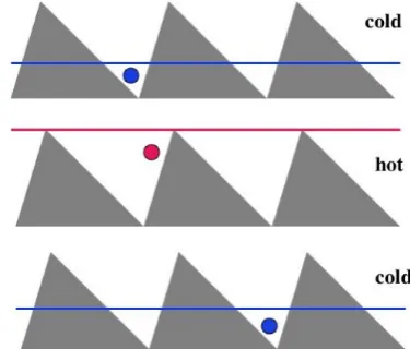
Fig. 9. A simple model of Brownian motor. Going from the top to the bottom of when the temperature is low (cold) a particle moving in the ratchet potential is trapped in one of the minima. Rising the temperature, the particle becomes almost free to move and, because its initial condition (minimum) is close the maximum on its right, the particle has more probability to go towards the right minimum. If the temperature is now decreased the particle has more probability to be trapped in the right minimum with respect being trapped in the minimum on the left.
Fig. 10. The Brownian motor proposed in Sect. 4. The particle moves in a periodic potential and noise is acting on it. A perturbing potential8(x−vt )localized in space is traveling in the system.
is now decreased the particle has more probability to be trapped in the right minimum with respect being trapped in the minimum to the left. The overall picture is that of a diffusion process with more probability to move to the right than on the left. Thus, under the combined action of periodic temperature variations and the ratchet potential, we can have a non zero drift average velocity of the particle in the right direction: we have been able to extract work from the temperature field.
There are many kinds of Brownian motors (Riemann and Hanggi, 2002), the one shown in Fig. 9 is just an example. We will propose here a new kind of motors using the very same idea of stochastic resonance to produce a non zero current using the noise. Instead of a ratchet potential, let us consider a particle which feel a space periodic potential of periodL. In the limit of overdamped friction, the equation of motion of the particle positionx is:
dx dt = −
∂V ∂x +
√
σ η(t ), V (x)=V0cos(2π x/L) (27)
We now introduce a time dependent forcingF (x−vt )in the form of a moving localized perturbation as shown in Fig. 10. Actually we can think of F (ξ ) as the effect of a moving potential perturbation, i.e.
F (x−vt )= −∂8(x−vt )
∂x . (28)
Without the effect of F, the particle performs a diffusive process among the minima of V. The characteristic time τL to jump to the right or to the left can be computed by
using the same method of Sect. 2. The action of the localized potential can introduce a new feature which is illustrated in Fig. 11.
Fig. 11. The effect of the perturbing potential8(x−vt ). From the top to the bottom, the particle can flip only in the positive x-direction as the potential travels. The flip occurs only for a suitable combination ofvand the noise amplitudeσ.
Fig. 12. The figure showsx(t )with (straight line) and without (dotted line)8(x−vt ) for a properly chosen value of σ. The initial particle position is 300Land the initial perturbing potential is localized inx=0.
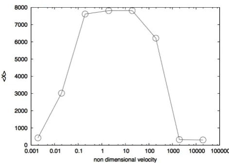
Fig. 13. The quantityhDxias a function ofσ.
Fig. 14. The quantityhDxias a function ofv.
When8is close tox=300, the particle remains trapped and it moves with the speed v for a rather long distance. At each step the particle is following the potential with a probability close to 1 but not exactly equal to 1. It follows that the particle is trapped in the potential8for a distance Dx which is a random variable (it is the analogous of the
random timeτLdiscussed in detail in Sect. 2).
As for the stochastic resonance, if the noise is too small or too large, 8 has no effect on the particle. The same is true if the velocity is too small or too large. We can check these qualitative statements in the following way. We consider an ensemble ofNparticles and we study the average distancehDxias a function of noise varianceσ and the non
dimensional velocityvτL/L. This is done in Figs. (13) and
(14), respectively.
In both cases, the effect of a resonant-like phenomenon is quite clear. Only for properly chosen values ofσ andv we do obtain the maximum ofhDxi. Some recent experimental
results (Schiavoni et al., 2002) seem to confirm the numerical analysis done in this section.
5 Conclusions
In the last 30 years the scientific community did learn many different features for complex systems, starting with the pioneering works of Lorenz, Ruelle, Mandelbrot and others. In many cases, new ideas and tools have been introduced in order to “measure” complexity in an appropriate way. These tools can be used to reveal different features of underlying physical or biological mechanisms. In some sense, stochastic resonance is also a tool because it allows us to understand whether or not non linear effects can act in a cooperative way with the complex and chaotic behavior of a given system. Note that stochastic resonance is a mechanism in the full meaning of the word because it allows to get large effect from a small amplitude perturbation. There have been and still are many applications of stochastic resonance to problems dealing with the amplification of signal to noise ratio, a quite traditional engineering problem.
In this paper, I have reviewed some known and less known features of stochastic resonance. Some simple conclusions can be made.
Stochastic resonance is a counter-intuitive phenomenon: it is not trivial that adding noise to a system we can enhance the deterministic periodic behavior.
Stochastic resonance is a robust mechanism, observed in many physical and biological systems. The notion of stochastic resonance is now cross disciplinary and new applications are found every year.
We learn a lot by applying stochastic resonance in the theory of climate change. As I mentioned in Sect. 2, it is a crucial step to understand that fast variables cannot simply be ignored in the study of long-term climatic change, which is, overall, the basic idea introduced by stochastic resonance.
Acknowledgements. I would like to thank many friends and
colleagues for their help in early days of my research in stochastic resonance. Among them a special mention must be made to Giorgio Parisi, Alfonso Sutera and Angelo Vulpiani. Also, I am indebted to Micheal Ghil and U. Frisch for their helps and contributions. This paper represents the talk I gave in april 2006 for the L. F. Richardson lecture at EGU annual meeting in Vienna. I would like to thank the scientific committee of the EGU Richardson’s medal and in particular D. Schertzer for his help and assistance. The paper has been written during a stay at the University of Chicago, Flash Center. I thank L. Kadanoff, D. Lamb, B. Fischer for their kind invitation and support.
Edited by: D. Schertzer
References
Alley, R. B., Anandankrishnan, S., and Jung, P.: Stochastic resonance in the North Atlantic, Paleoceanography, 16, 190–198, 2001.
Benzi, R.: Flow Reversal in a Simple Dynamical Model of Turbulence, Phys. Rev. Lett., 95, 024502, doi:10.1103/PhysRevLett.95.024502, 2005.
Benzi, R. and Sutera, A.: Turbulence and Predictability in Geophysical Fluid Dynamics and Climate Dynamics, edited by: Ghil, M., Benzi, R., and Parisi, G., Varenna Summer School LXXXVIII 1983, 1985.
Benzi, R. and Sutera, A.: Stochastic resonance in two-dimensional Landau Ginzburg equation, J. Phys. A, 37, L391, doi:10.1088/0305-4470/37/32/L01, 2004.
Benzi, R., Sutera, A., and Vulpiani, A.: The mechanism of stochastic resonance, J. Phys. A, 14, L453, doi:10.1088/0305-4470/14/11/006, 1981.
Benzi, R., Parisi, G., Sutera, A., and Vulpiani, A.: Stochastic resonance in climatic change, Tellus, 34, 10–16, 1982.
Benzi, R., Jona-Lasinio, G., and Sutera, A.: Stochastically perturbed Landau-Ginzburg equations, J. Stat. Phys., 55(3–4), 505–522, doi:10.1007/BF01041596, 1989.
Bulsara, A., Hanggi, P., Marchesoni, F., Moss, F., and Schlesinger, M. (Eds.): Stochastic Resonance in Physics and Biology, J. Stat. Phys., 70, 1–512, 1993.
Feynman, R. P., Leighton, R. B., and Sands, M.: The Feynman Lectures on Physics, Addison Wesley, Reading MA, 1, Chap. 46, 1963.
Giammaitoni, L., Hanggi, P., Jung, P., and Marchesoni, F.: Stochastic resonance, Rev. Mod. Phys., 70, 223, doi:10.1103/RevModPhys.70.223, 1996.
McNamara, B. and Wiesenfeld, K.: Theory of stochastic resonance, Phys. Rev. A., 39, 4854–4869, doi:10.1103/PhysRevA.39.4854, 1989.
Moss, F. and Wiesenfeld, K.: The benefits of background noise, Sci. Am., 273, 66–69, 1995.
Nicolis, C.: Solar variability and stochastic effects on climate, Sol. Phys., 74(2), 473–478, doi:10.1007/BF00154530, 1981. Nicolis, C.: Stochastic aspects of climatic transitions – response to
a periodic forcing, Tellus, 34, 1–9, 1982.
Parrondo, J. M. R. and Cisneros, B. J.: Finite-time Thermodynam-ics and ThermoeconomThermodynam-ics, Appl. Phys. A, 75, 179–191, 2002. Ganopolski, A. and Rahmstorf, S.: Abrupt glacial climate changes
due to stochastic resonance. Phys. Rev. Lett., 88, 038501-1– 038501-4, 2002.
Riemann, P. and Hanggi, P.: Introduction to the physics of Brownian motors, Appl. Phys. A, 75, 169–178, 2002.
Schiavoni, M., Carminati, F.-R., Sanchez-Palencia, L., Renzoni, F., and Grynberg, G.: Stochastic resonance in periodic potentials: Realization in a dissipative optical lattice, Europhys. Lett., 59, 493, doi:10.1209/epl/i2002-00134-y, 2002.