www.nonlin-processes-geophys.net/14/395/2007/ © Author(s) 2007. This work is licensed
under a Creative Commons License.
Nonlinear Processes
in Geophysics
Merging particle filter for sequential data assimilation
S. Nakano1,2, G. Ueno1,2, and T. Higuchi1,2
1The Institute of Statistical Mathematics, Research Organization of Information and Systems, Japan 2Japan Science and Technology Agency, Japan
Received: 8 January 2007 – Revised: 25 April 2007 – Accepted: 5 July 2007 – Published: 16 July 2007
Abstract. A new filtering technique for sequential data
as-similation, the merging particle filter (MPF), is proposed. The MPF is devised to avoid the degeneration problem, which is inevitable in the particle filter (PF), without pro-hibitive computational cost. In addition, it is applicable to cases in which a nonlinear relationship exists between a state and observed data where the application of the ensemble Kalman filter (EnKF) is not effectual. In the MPF, the filter-ing procedure is performed based on samplfilter-ing of a forecast ensemble as in the PF. However, unlike the PF, each mem-ber of a filtered ensemble is generated by merging multiple samples from the forecast ensemble such that the mean and covariance of the filtered distribution are approximately pre-served. This merging of multiple samples allows the degen-eration problem to be avoided. In the present study, the newly proposed MPF technique is introduced, and its performance is demonstrated experimentally.
1 Introduction
Data assimilation is performed to obtain the best estimates of a state of a dynamic system or the evolution of a system by incorporating observation into a model of the system and is used as an important tool for modeling and prediction of geophysical processes. Data assimilation methods are clas-sified into two categories: variational data assimilation and sequential data assimilation. While variational data assimi-lation is performed by fitting a dynamic model to all of the available observations during a period of interest, sequential data assimilation is an on-line approach that updates the es-timation of a state at each observation time. In the present study, we focus on sequential data assimilation.
Correspondence to: S. Nakano ([email protected])
Most sequential data assimilation techniques basically consider a probability density function (PDF) of a state of a dynamic system. An assimilation process is based on a prior PDF of the current state which is obtained using past data and a system model. This prior PDF is then updated to obtain the posterior PDF of the state by incorporating con-straints based on observation. The procedure used to obtain the posterior PDF is called “filtering”. The filtering proce-dure provides a PDF of the current state considering current and past observations, which should be a basis for accurate prediction of future states.
If a PDF of a state is Gaussian and the dynamics of the system is linear, then a filtering process can be described by the algorithm of the Kalman filter. However, since geophys-ical systems usually contain inherent nonlinearity, it is rare that the Kalman filter can be applied. The Kalman filter al-gorithm is sometimes extended by modifying the calculation of covariances of a state by linearizing a system model, and this extended algorithm is called the extended Kalman filter (EKF). However, for models with high nonlinearity, the EKF can make errors diverge (e.g., Evensen, 1992). Moreover, for a model with a large number of variables, the EKF requires a high computational cost. Although the computational cost could be reduced by using a variant of the EKF, the singu-lar evolutive extended Kalman (SEEK) filter (Pham et al., 1998b), the SEEK filter also requires the linearization of a system model and it can provide an unstable result for cases with high nonlinearity.
Kalman gain calculated from the mean and the covariances of the prior ensemble. However, the EnKF basically assumes a linear relationship between a state and observed data in cal-culating a Kalman gain. Therefore, the EnKF does not pro-vide good estimates of a state for cases in which linear ap-proximation of the relationship between a state and observed data is invalid. In addition, the computational cost of each filtering step in the EnKF is large due to repetitive multipli-cations and additions of matrices. Pham et al. (1998a) have proposed another ensemble-based filtering method, the sin-gular evolutive interpolated Kalman (SEIK) filter, which is derived as a variant of the SEEK filter. Although the SEIK filter can work more efficiently than the EnKF (Nerger et al., 2005), it is not applicable to cases with nonlinear observation as well.
The particle filter (PF) (Gordon et al., 1993; Kitagawa, 1993, 1996; Kitagawa and Gersch, 1996; Higuchi and Kita-gawa, 2000; van Leeuwen, 2003), which is sometimes re-ferred to as the sequential importance resampling (SIR) fil-ter, is another method that is based on ensemble approxima-tion of a PDF. In the PF, an estimaapproxima-tion of a posterior PDF is obtained by resampling with replacement from a prior en-semble. As the PF does not require assumptions of linearity or Gaussianness, it is applicable to general nonlinear prob-lems. In particular, the PF can be applied to cases in which the relationship between a state and observed data is nonlin-ear, to which the application of the ensemble Kalman filter (EnKF) is not appropriate. However, the PF often encounters a problem called “degeneration”, which does not occur in the EnKF. Since resampling procedures are applied recursively, most of the particles are replaced by particles that fit the ob-served data better, and the posterior PDF is eventually rep-resented by only a few of the particles among the members of the initial ensemble. This reduces the validity of ensemble approximation. This problem could be avoided by increasing the number of particles in the ensemble. However, in order to increase the number of particles, a prohibitive computational cost is often required at each forecast step.
One potential way to avoid the degeneration problem is to approximate a posterior distribution as a Gaussian distri-bution. This approach has been proposed by Kotecha and Djuri´c (2003) under the name of the Gaussian particle filter (GPF), and a similar algorithm was also presented by Ander-son and AnderAnder-son (1999). In this technique, from an ensem-ble that represents a filtered posterior distribution, the mean and covariances are calculated to obtain a Gaussian distribu-tion for approximating the filtered distribudistribu-tion. By drawing random samples from this Gaussian distribution, a filtered ensemble is newly generated. In the GPF, although the ac-curacy of an approximation of a filtered distribution is worse than in the PF because of the assumption of Gaussianness, no duplicate particles are contained in the ensemble and de-generation does not occur. However, in generating Gaussian random vectors to make a Gaussian ensemble, we must fac-torize the covariance matrix, which requires a high
computa-tional cost if the dimension of a state vector is large. In most practical cases, factorization of the covariance matrix with the dimension of a state vector is not realistic.
There is another way to avoid degeneration which is a vari-ant of the PF referred to as the kernel filter (H¨urzeler and K¨unsch, 1998; Anderson and Anderson, 1999) or the regu-larized particle filter (Musso et al., 2001). This technique approximates the filtered PDF by a sum of Gaussian func-tions with small standard deviafunc-tions centered at the particle locations, and members of a filtered ensemble is drawn from the sum of Gaussian functions. However, in applying this technique to high-dimensional models, there is difficulty in designing a covariance matrix for each of the Gaussian func-tions. Although a covariance matrix could be made on the basis of the covariance matrix of an ensemble representing a prior or posterior PDF, this bring the same problem as the GPF; that is, the factorization of the covariance matrix is re-quired and the computational cost would become prohibitive in cases that a state vector is high-dimensional.
Thus, there exists no practical method to allow sequential data assimilation with acceptable computational cost, except some methods such as the EnKF and the SEIK filter which also have a disadvantage in that it is not necessarily appli-cable to cases with nonlinear observations. To overcome this problem, another technique, the merging particle filter (MPF), is devised. The MPF is an improved algorithm of the PF, in which filtering is performed by merging several parti-cles of a prior ensemble, which is rather similar to the genetic algorithm (e.g., Goldberg, 1989). This merging procedure al-lows the degeneration problem to be avoided and requires far fewer particles than the PF. The primary advantage of the PF over the EnKF is inherited; that is, the MPF is applicable even to cases in which the relationship between a state and observed data is nonlinear. Moreover, since the MPF does not require the calculation of an inverse matrix, the compu-tational cost at each filtering step is lower than that of the EnKF. The PF algorithm, which the proposed algorithm is based on, is reviewed in Sect. 2, and the MPF algorithm is introduced in Sect. 3. In order to evaluate the performance of the MPF, the results of a number of experiments are de-scribed in Sect. 4. Finally, the effectiveness of the MPF is discussed and summarized in Sect. 5.
2 Particle filter
The following state space model is considered:
xk =Fk(xk−1,vk) (1a)
yk=Hk(xk)+wk (1b)
the temporal evolution of a state from timetk−1to timetk ac-cording to the system model based on the simulation, while Hk projects the state vectorxkto the observation space.
The PF considers a PDF of a state xk, and the PDF is approximated by an ensemble consisting of a large num-ber of discrete samples called ‘particles’. For example, a filtered distribution at timeT=tk−1,p(xk−1|y1:k−1), is ap-proximated by particles{x(1)k−1|k−1,x(2)k−1|k−1,· · · ,x(N )k−1|k−1}
as
p(xk−1|y1:k−1)≈ 1 N
N X
i=1
δxk−1−x(i)k−1|k−1
(2)
where δ is Dirac’s delta function, and N is the num-ber of particles in the ensemble. Here we expressed p(xk−1|y1,· · ·,yk−1)asp(xk−1|y1:k−1). From this
ensem-ble approximation ofp(xk−1|y1:k−1), we obtain an ensemble
approximation of the forecast distribution of the state at the next observation timeT=tkas
p(xk|y1:k−1)≈
1 N
N X
i=1
δxk−x(i)k|k−1
. (3)
Each particle of the forecast ensemble x(i)k|k−1 is given by Fk(x(i)k−1|k−1,v
(i)
k )wherev (i)
k is a realization of the system noise. This procedure is called the forecast step.
From the forecast distributionp(xk|y1:k−1)and observed datayk, we obtain a filtered PDFp(xk|y1:k)by using Bayes’ theorem, as follows:
p(xk|y1:k)
= R p(xk|y1:k−1) p(yk|xk)
p(xk|y1:k−1) p(yk|xk)dxk
≈ 1
P jp
yk|x(j )k|k−1
N X
i=1
pyk|x(i)k|k−1
δxk−x(i)k|k−1
=
N X
i=1 wiδ
xk−x(i)k|k−1
(4) wherep(yk|x(i)k|k−1)is the likelihood ofx
(i)
k|k−1given the data
ykand the weightwiis defined as
wi =
p(yk|x(i)k|k−1)
P
jp(yk|x(j )k|k−1)
. (5)
This is called the filtering step.
Equation (4) shows thatp(xk|y1:k)is approximated using particles weighted bywi. Based on Eq. (4), we obtain a new ensemble {x(1)k|k,· · · ,x(N )k|k}which approximatesp(xk|y1:k) by resampling the forecast ensemble {x(1)k|k−1,· · ·,x(N )k|k−1}
with a weight of wi for each i. The new ensemble may
contain multiple copies ofx(i)k|k−1 belonging to the forecast ensemble, and the number of copiesmi becomes
mi ≈N wi X
mi =N; mi ≥0
(6)
for eachx(i)k|k−1. From Eqs. (4) and (6), we obtain an approx-imation ofp(xk|y1:k)using uniformly weighted particles, as follows:
p(xk|y1:k)≈ N X
i=1 wiδ
xk−x(i)k|k−1
≈
N X
i=1 mi N δ
xk−x(i)k|k−1
= 1
N N X
i=1
δxk−x(i)k|k
.
(7)
Thus, the newly generated ensemble approximates the fil-tered PDFp(xk|y1:k). Equation (7) has the same form as Eq. (2), which allows us to recursively repeat the above pro-cedure from Eq. (2) to Eq. (7). By repeating the propro-cedure, a sequence of observed data is incorporated into the system model.
3 Merging particle filter
In the PF, a filtered ensemble generated through the resam-pling procedure contains multiple copies of particles with high likelihoods, and particles with low likelihoods are re-moved from the ensemble. Therefore, after repeating resam-pling several times, the diversity of the ensemble decreases and eventually becomes insufficient for validly representing a PDF. This problem can be avoided by increasing the num-ber of particles. However, due to limited computational re-sources, it is often impossible to use a sufficient number of particles to repeat resampling several times. The MPF, which we propose in this section, allows us to remake a filtered en-semble while restraining the reduction of its diversity.
The MPF is a modification of the PF. In the MPF, a filtered ensemble is constructed based on samples from a forecast semble as in the PF. However, each particle of a filtered en-semble is generated as an amalgamation of multiple particles from the forecast ensemble, which is rather similar to the ge-netic algorithm. Although this does not ensure that the shape of the filtered PDF is preserved, the mean and covariance of the filtered PDF are approximately preserved (asymptotically preserved as the number of particles approaches infinity) in generating a filtered ensemble.
{ ˆx(j,1)k|k ,· · ·,xˆ(j,N )k|k }from then×N samples forms an en-semble approximating the filtered PDF, which satisfies
p(xk|y1:k)≈ 1 N
N X
i=1
δxk− ˆx(j,i)k|k (8)
because it consists of N samples drawn from the forecast ensemble with weights ofwi, as was the case in obtaining the filtered ensemble in the previous section. Next, we make a new ensemble consisting ofNparticles{x(1)k|k,· · · ,x(N )k|k}to approximatep(xk|y1:k). Each particle in the new ensemble is generated as a weighted sum ofnsamples from then×N sample set as:
x(i)k|k=
n X
j=1
αjxˆ(j,i)k|k . (9)
In order to ensure that the newly generated ensemble pre-serves the mean and covariances of the filtered PDF for N→∞, the merging weightsαjare set to satisfy
n X
j=1
αj =1 (10a)
n X
j=1
α2j =1 (10b)
where eachαj is a real number. When the merging weights satisfy Eq. (10a), the mean of the PDF approximated by the new ensemble{x(1)k|k,· · ·,x(N )k|k}becomes
Z xk 1 N N X
i=1 δ
xk−x(i)k|k
dxk
= 1
N N X
i=1
x(i)k|k = 1
N N X
i=1 n X
j=1 αjxˆ(j,i)k|k
=
n X
j=1 "
αj Z
xk 1
N N X
i=1
δxk− ˆx(j,i)k|k dxk
#
≈
n X
j=1 αj
Z
xkp(xk|y1:k) dxk
= Z
xkp(xk|y1:k) dxk=µk|k
(11)
whereµk|k is the mean of the filtered PDFp(xk|y1:k). In addition, if the merging weightsαj satisfy Eq. (10b), the
co-variances given by the new ensemble become Z
(xk−µk|k)(xk−µk|k)T 1 N
N X
i=1
δxk−x(i)k|k
dxk
=1
N N X
i=1
(x(i)k|k−µk|k)(x(i)k|k−µk|k)T
=1
N N X
i=1 n X
j1=1
αj1xˆ(j1k|k,i)−µk|k ! n
X
j2=1
αj2xˆ(j2,i)k|k −µk|k !T
=1
N N X
i=1
" n X
j1=1 αj1
ˆ x(j1,i)
k|k −µk|k
#" n X
j2=1 αj2
ˆ x(j2,i)
k|k −µk|k #T ≈1 N N X
i=1 n X
j=1
α2jxˆ(j,i)k|k −µk|k xˆ(j,i)k|k −µk|k T
=
n X
j=1 α2j
Z
(xk−µk|k)(xk−µk|k)T 1 N
N X
i=1
δxk− ˆx(j,i)k|k
dxk
≈ Z
(xk−µk|k)(xk−µk|k)T p(xk|y1:k) dxk=6k|k
(12) where6k|kis the covariance matrix ofp(xk|y1:k). Here, we
used an approximation as 1
N N X
i=1 (xˆ(j1,i)
k|k −µk|k)(xˆk(j|2k,i)−µk|k)T ≈0 (ifj16=j2),
which is justified because the two sets of samples
{ ˆx(j1,1) k|k ,· · ·,xˆ
(j1,N ) k|k }and{ ˆx
(j2,1) k|k ,· · · ,xˆ
(j2,N )
k|k }are obtained through independent random sampling and would not corre-late with each other. Therefore, the ensemble obtained using Eq. (9) affords an approximation of p(xk|y1:k)preserving the mean and covariances as
p(xk|y1:k)≈
1 N
N X
i=1 δ
xk−x(i)k|k
. (13)
The number of merged particlesncan be chosen almost arbitrarily. However, in order that the merging procedure makes sense,nmust be equal to or greater than 3. Ifn=1, the weightα1 must be 1 in order to satisfy both Eqs. (10a) and (10b), which is obviously equivalent to the normal PF. If n=2, then one of merging weights must be 1, and the other must be 0, so as to satisfy both Eqs. (10a) and (10b). This setting is also equivalent to the normal PF, which means that the merging procedure does not make sense. Although there is no upper limit forn, it is not necessary to setnto be large. As shown in the next section, if none of the merging weights are zero, we would greatly benefit by the merging procedure even whennis as small as 3.
Resampling (
N
particles)
Forecast ensemble (
N
particles)
Forecast ensemble (
N
particles)
State
x
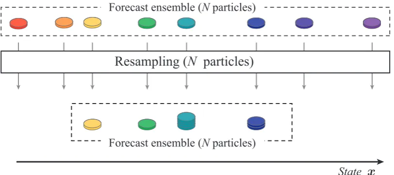
Fig. 1. PF scheme. The value of a statexis on the horizontal axis assuming that the statexis scalar.
the weights, it would be preferable to set them such that no two weights are equal to each other and that none of the weights become zero in order to reinforce the diversity of the filtered ensemble. Under this setting, two duplicate particles in the filtered ensemble {x(1)k|k,· · ·,x(N )k|k} can be generated only from two identical sets of n merged parti-cles drawn from the forecast ensemble{x(1)k|k−1,· · ·,x(N )k|k−1}, if duplicate particles are not contained in the forecast en-semble. When the probability that particlex(i)k|k−1is drawn from the forecast ensemble iswi (0≤wi<1), the probability that a sequence ofnparticles{x(i1)k|k−1,· · · ,x(in)
k|k−1}is drawn is Qn
j=1wij. Since
Qn
j=1wij≤(maxwi)
n, the number of duplicate particles contained in the filtered ensemble is, at most, approximatelyN×(maxwi)nfor the MPF, while it is N×maxwi for the PF.
Figures 1 and 2 show schematically the respective proce-dures of the PF and the MPF when the number of merging particles is set to be 3. In the PF, a filtered ensemble is sim-ply obtained by resampling. In the MPF with 3 merging par-ticles, after 3N particles are sampled from the forecast en-semble, the 3N particles are divided into N combinations of 3 particles, and the 3 particles in each combination are merged to obtain a new particle. Even from combinations of the same 3 particles, different particles can be made with dif-ferent sets of weights. Thus, the filtered ensemble obtained with the MPF contains diverse particles in comparison with that obtained with the PF.
4 Numerical experiments
4.1 Lorenz 63 model
We performed a numerical experiment to test the MPF. Al-though this method is actually devised for data assimilation for high-dimensional models, we first used a simple model, the Lorenz 63 model (Lorenz, 1963), to investigate the be-haviors of the method. The Lorenz 63 model is described by the following equations:
dx
dt = −s(x−y) (14a)
dy
dt =rx−y−xz (14b)
dz
dt =xy−bz. (14c)
In the conventional parameter setting, the three parameters are set as follows: s=10,r=28, andb=8/3. One time step in integrating the system equation was set to be 0.01.
Initially, we ran this model to generate a sequence of mea-surement data for this test. The data were generated every 20 time step with errors of a standard deviation of 2.0. It was as-sumed that all of the components of the state vector,x,y, and z, could be observed. In this situation, the observation vector at each observation time resides in the same vector space as the state vector.
The generated data were assimilated into the model using the PF and the MPF. In this and the following experiments, we assume additive system noise, and thus Eqs. (1a) and (1b) are rewritten as follows.
xk =F (xk−1)+vk (15a)
Merging
Resampling (3
N
particles)
Forecast ensemble (
N
particles)
Forecast ensemble (
N
particles)
State
x
Fig. 2. Scheme of the MPF, in which the number of merging particles is set to be 3. The value of a statexis on the horizontal axis assuming that the statexis scalar.
where the subscriptk inFk andHk is omitted because the system and observation models considered here are time-independent. In applying the MPF, the number of merged particles was set ton=3, and the weightsαj were set as fol-lows:
α1=3
4 (16a)
α2= √
13+1
8 (16b)
α3= − √
13−1
8 (16c)
which satisfies Eqs. (10a) and (10b). In both the PF and the MPF, we need to calculate the likelihood p(yk|xk) where
yk is the observation vector(xko, yko, zok), andxk is the state vector(xk, yk, zk)at timeT=tk. Assuming that observation noisewk obeys a Gaussian distribution with zero mean and a diagonal covariance as diag(σ2, σ2, σ2), the likelihood be-comes
p(yk|xk)= 1
√
2π σ exp "
−||yk−xk||
2
2σ2 #
(17)
where we setσ=3. The system noise was assumed to be a Gaussian noise with zero mean and a diagonal covariance as
diag(0.01,0.01,0.01). Particles of the forecast ensemble at the initial time step (T=t1) were generated from a Gaussian distribution where the mean was given by the value of the data at the same time step and the standard deviation was 4.0 for each component.
-30 -20 -10 0 10 20 30
0 2000 4000 6000 8000 10000 Step
State MPF Data
Fig. 3. Result of the experiment of data assimilation by the MPF
for the Lorenz 63 model. The number of particles was set toN=64. The black squares indicate the test data that were assimilated into the model. The red line indicates the true state ofx, and the blue line indicates the estimation ofxas a result of the data assimilation.
-30 -20 -10 0 10 20 30
0 2000 4000 6000 8000 10000
Step
State PF Data
Fig. 4. Result of the experiment of data assimilation by the PF for
the Lorenz 63 model. The number of particles was set toN=64. The black squares indicate the test data that were assimilated into the model. The red line indicates the true state ofxand the blue line indicates the estimation ofxas a result of the data assimilation.
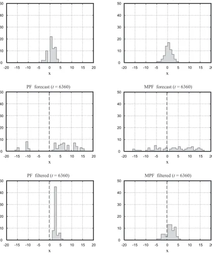
In order to clarify why the PF failed to trace the true tra-jectory, histograms of the ensemble forx around time step 6360 are shown in Fig. 7. At time step 6340, a gap appeared around−1<x<0 in the filtered ensemble in the result by the PF. This gap expanded remarkably at the next forecast step, resulting in a large gap in the forecast ensemble at time step 6360. While thexvalue of the true state was−0.125 at this time step, as indicated by the dashed line in each panel, no members of the ensemble were distributed around the true state. In contrast, no distinct gap appeared in the filtered en-semble at time step 6340 in the result obtained by the MPF. Thus, there were only small gaps in the forecast ensemble at the next time step.
-30 -20 -10 0 10 20 30
6000 6200 6400 6600 6800 7000
Step
State MPF Data
Fig. 5. Result of the experiment of data assimilation by the MPF
for the Lorenz 63 model from time step 6000 to time step 7000 for the x-component.
-30 -20 -10 0 10 20 30
6000 6200 6400 6600 6800 7000
Step
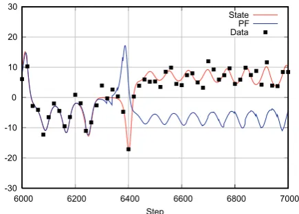
State PF Data
Fig. 6. Result of the experiment of data assimilation by the PF for
the Lorenz 63 model from time step 6000 to time step 7000 for the x-component.
0 10 20 30 40 50
-20 -15 -10 -5 0 5 10 15 20
x
0 10 20 30 40 50
-20 -15 -10 -5 0 5 10 15 20
x
0 10 20 30 40 50
-20 -15 -10 -5 0 5 10 15 20
x
0 10 20 30 40 50
-20 -15 -10 -5 0 5 10 15 20
x
0 10 20 30 40 50
-20 -15 -10 -5 0 5 10 15 20
x
0 10 20 30 40 50
-20 -15 -10 -5 0 5 10 15 20
x
PF filtered (t = 6340)
PF forecast (t = 6360)
PF filtered (t = 6360)
MPF filtered (t = 6340)
MPF forecast (t = 6360)
MPF filtered (t = 6360)
Fig. 7. Histograms of the distribution ofxin the ensemble around time step 6360. The left-hand panels show the distributions for the results obtained by the PF, and the right-hand panels show the distributions for the results obtained by the MPF. The upper panels show the filtered distributions at time step 6340. The middle panels show the forecast distributions at time step 6360. The lower panels show the filtered distribution at time step 6360. In the middle and lower panels, for reference, the true state ofxis indicated with dashed lines.
4.2 Lorenz 96 model
In order to evaluate the performance of the MPF for models on higher dimension, we performed another experiment
us-ing the Lorenz 96 model (Lorenz and Emanuel, 1998), which is described by the following equations:
dxj
Table 1. Root-mean-square deviations from the true state over
50 000 time steps for an experiment using the Lorenz 63 model.
PF MPF EnKF
N=64 4.55 1.00 1.34
N=128 3.87 0.91 1.29
N=256 0.87 0.92 1.29
N=512 0.86 0.91 1.29
Table 2. Root-mean-square deviations from the true state from time
step 3000 to time step 20 000 for an experiment using the Lorenz 96 model. Since the result has converged to the limit, we omitted to calculate the deviations forN >8192 for the EnKF and those for N >65 536 for the MPF.
PF MPF EnKF
N=128 3.47 1.74 0.91
N=256 3.10 1.03 0.88
N=512 2.94 0.90 0.87
N=1024 2.26 0.84 0.87
N=2048 1.60 0.83 0.86
N=4096 1.29 0.81 0.86
N=8192 1.08 0.81 0.86
N=16 384 0.96 0.80 –
N=32 768 0.84 0.80 –
N=65 536 0.83 0.80 –
N=131 072 0.79 – –
N=262 144 0.77 – –
forj=1, . . . , J. Here,x−1=xJ−1,x0=xJ, andxJ+1=x1. In this study,Jwas set to be 40; that is, the dimension of a state vector is 40. The forcing termf was set to be 8. One time step was set to be 0.005. In order to generate data for the experiment, we ran this model from the initial condition as
xj =8.0 (forj 6=20) (19a)
xj =8.008 (forj =20). (19b)
After we iterated the model through 2000 time steps to al-low fluctuations in the system to develop sufficiently, the data were generated every 10 time steps with errors hav-ing a standard deviation of 1.5. It was assumed that we can observexj ifj is an even number (j=2, . . . ,40); that is, if half of the state variables are observed. In assimilat-ing these test data, the system noise was assumed to be a Gaussian noise with zero mean and a diagonal covariance as diag(0.25, . . . ,0.25). Particles of the forecast ensemble at the initial time step (T=t1) were generated from a Gaussian distribution with mean 2.0 and variance 2.0 for each com-ponent. Again, in applying the MPF, the number of merged particles was set ton=3, and the weightsαjwere set accord-ing to Eq. (16). The likelihood was calculated as follows:
0 10 20 30 40
10000 9000 8000 7000 6000 5000 4000 3000
j
Time step
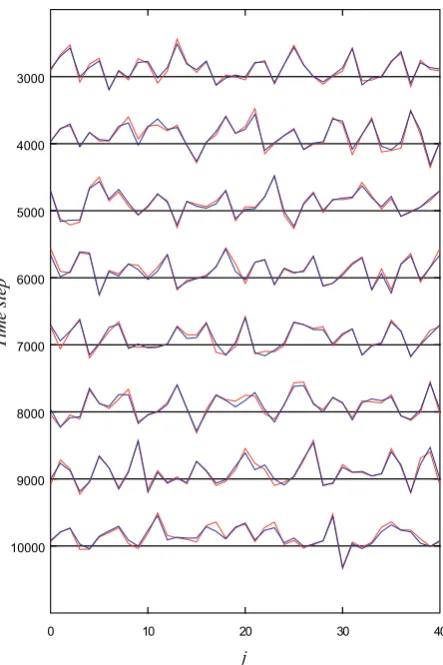
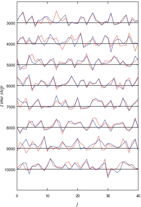
Fig. 8. Result of the experiment of data assimilation by the MPF for
the Lorenz 96 model for every 1000 times step from 3000 to 10 000. In this experiment, the number of particles was set toN=512. The red and blue lines indicate the true state and the estimate by the MPF, respectively.
p(yk|xk)= 1
√
2π σ exp "
−||yk−Hxk||
2
2σ2 #
(20)
where yk is the observation vector (y1,k, . . . , y20,k) and σ was set to be 3. The operator H extracts the observ-able components from the state vector xk. Since we as-sume that we can observe xj for an even number of j, Hxk=(x2,kx4,k. . . x40,k)T.
0 10 20 30 40 10000
9000 8000 7000 6000 5000 4000 3000
j
Time step
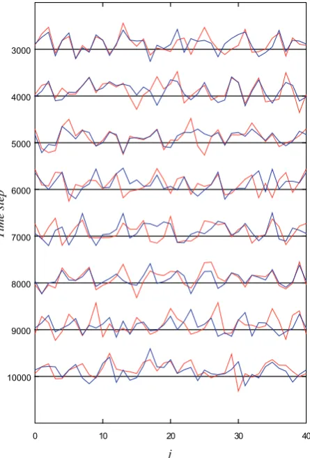
Fig. 9. Result of the experiment of data assimilation by the PF for
the Lorenz 96 model for every 1000 time steps from 3000 to 10 000. In this experiment, the number of particles was set toN=512. The red and blue lines indicate the true state and the estimate by the PF, respectively.
the true state from time step 3000 to time step 20 000 for various numbers of particles. Again, for reference purposes, the results using the EnKF are also shown in this table. We omitted the calculation of the deviations forN >8192 for the EnKF and those forN >65 536 for the MPF which requires much computational resources and cost, because the value of the root-mean-square deviation has converged to the limit and the estimate would not be improved any more even ifN increased.
WhenNis small, the MPF fails to estimate the state, while the EnKF achieves a robust estimation of the state. However, the estimation accuracy of the MPF is remarkably improved whenN=256, and it becomes better than that of the EnKF whenN≥1024. In comparison with the PF, the MPF pro-vides good estimates without requiring a large number of par-ticles. In this experiment, the MPF requires only 1024 cles to obtain as good accuracy as the PF with 32 768 parti-cles. As the number of ensemble membersN increases, the
result using the PF is gradually improved, and the root-mean-square of the deviations for the PF seems to converge to a slightly better value than that for the MPF, probably because the MPF does not preserve the shape of the PDF while the PF can faithfully preserve the shape of the filtered PDF with abundant particles. For cases thatN is larger than 262 144, we did not perform experiments because they need too much computational resources, and we could not confirm the value which the root-mean-square deviation for the PF converged to. Thus, the result of the PF with a further large ensemble size possibly converges to a further good value than that for N=262 144. However, the use of such an enormous number of particles is not realistic, and it seems to provide only minor improvement of the estimation accuracy even if it were possi-ble. For practical applications to high-dimensional systems, the use of the MPF or the EnKF with much fewer particles would be effectual.
4.3 Lorenz 96 model with nonlinear observation
Another experiment was performed to examine whether the MPF works for the Lorenz 96 model with nonlinear obser-vations. In this experiment, we assumed that we can ob-serve only an absolute value |xj| if j is an even number (j=2, . . . ,40). The data were generated every 10 time steps by taking the absolute values ofxj containing errors with a standard deviation of 1.5. As in the previous experiment, the system noise was assumed to be a Gaussian noise with zero mean and a diagonal covariance as diag(0.25, . . . ,0.25), and particles of the forecast ensemble at the initial time step (T=t1) were generated from a Gaussian distribution with mean 2.0 and variance 2.0 for each component. The num-ber and the weights of the merged particles in applying the MPF were also the same as in the previous experiment. The likelihood was calculated as follows:
p(yk|xk)= 1
√
2π σ exp "
−||yk−H (xk)||
2
2σ2 #
(21)
0 10 20 30 40 10000
9000 8000 7000 6000 5000 4000 3000
j
Time step
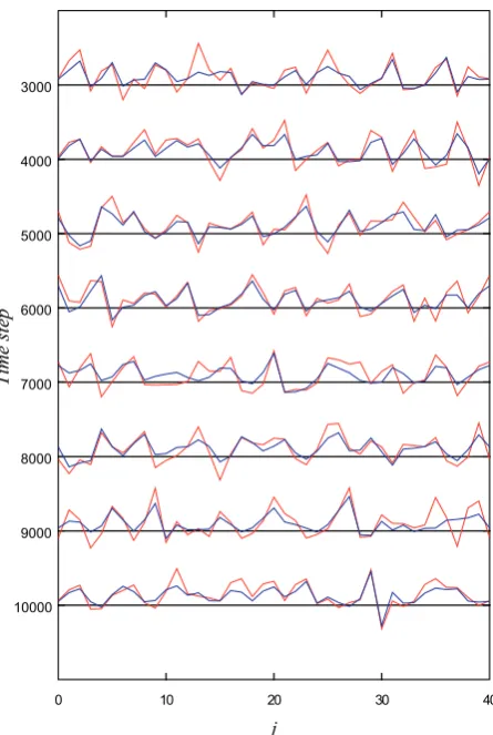
Fig. 10. Result of the experiment of data assimilation by the MPF
for the Lorenz 96 model with nonlinear observations for every 1000 time steps from 3000 to 10 000. In this experiment, the number of particles was set toN=1024. The red and blue lines indicate the true state and the estimate by the MPF, respectively.
(2003), we define a new state vectorx0
k=[xTk, (H (xk))T]T such that the observation model becomes linear, and the state space model in Eqs. (15a) and (15b) is accordingly rewritten into a new state space model as follows:
x0k=F0(x0k−1,vk) (22a)
yk=H0x0k+wk. (22b)
Here the operatorsF0andH0are defined as: F0(x0k−1,vk)=F0 xk−1, H (xk−1),vk
=
F (xk−1)+vk H F (xk−1)+vk
(23a)
H0=(Odimxk Idimyk) (23b)
whereOdimxk is a zero matrix whose dimension is the same
as xk andIdimyk is an identity matrix whose dimension is
0 10 20 30 40
10000 9000 8000 7000 6000 5000 4000 3000
j
Time step
Fig. 11. Result of the experiment of data assimilation by the PF
for the Lorenz 96 model with nonlinear observations for every 1000 time steps from 3000 to 10 000. In this experiment, the number of particles was set toN=1024. The red and blue lines indicate the true state and the estimate by the PF, respectively.
the same asyk, and thusH0extractsH (xk)from the vector
x0k. The EnKF is then applied to this new state space model. Since the results have converged to the limit, we omitted to calculate the deviations forN >8192 for the EnKF and those forN >65 536 for the MPF.
Table 3. Root-mean-square deviations from the true state from time
step 3000 to time step 20 000 for an experiment using the Lorenz 96 model with nonlinear observation. Since the result has converged to the limit, we omitted to calculate the deviations forN >8192 for the EnKF and those forN >65 536 for the MPF.
PF MPF EnKF
N=128 4.17 3.56 1.75
N=256 4.01 2.47 1.94
N=512 3.66 1.50 1.93
N=1024 3.70 1.20 1.98
N=2048 3.15 1.19 1.99
N=4096 2.65 1.14 1.99
N=8192 2.07 1.14 1.99
N=16 384 1.80 1.13 –
N=32 768 1.23 1.13 –
N=65 536 1.19 1.13 –
N=131 072 1.04 – –
N=262 144 1.00 – –
accuracy than the MPF. Thus, as far as the number of parti-cles is not allowed to increased to more than at least 65 536, the degeneration problem of the PF is more serious than the problem concerning high order moments of the MPF in this experiment. In comparison between the MPF and the EnKF, whenNis small, the EnKF provides better estimations again, although estimations by the EnKF are not so good. When N≥512, the estimation accuracy of the MPF is remarkably improved to be much better than that of the EnKF. Actually, the EnKF does not effectively work in this experiment. Fig-ure 12 shows the estimation by the EnKF, where the number of particles was set toN=1024. It is indicated that the esti-mates by the EnKF often significantly deviate from the true state which means that the EnKF fails to capture the varia-tion of the true state. Thus, for this experiment, the use of the MPF would be the most effectual.
5 Summary and discussion
We proposed a new algorithm, the MPF, for realizing prac-tical sequential data assimilation. The MPF provides an ensemble-based approximation of the filtered PDF such that the mean and covariance are approximately preserved. The MPF allows the problem of degeneration, which occurs in the PF, to be avoided. It must be noted that the MPF does not preserve the shape of the filtered PDF while the PF can faithfully preserve the shape of the filtered PDF with abun-dant particles. Therefore, if a sufficient number of particles is used, the PF should provide a better estimation than the MPF. In particular, in cases that the filtered PDF is signifi-cantly non-Gaussian, the MPF possibly provides a rather bad estimate. In application to a high-dimensional system, how-ever, it is not realistic to use a sufficient particles to avoid
de-0 10 20 30 40
10000 9000 8000 7000 6000 5000 4000 3000
j
Time step
Fig. 12. Result of the experiment of data assimilation by the EnKF
for the Lorenz 96 model with nonlinear observations for every 1000 time steps from 3000 to 10 000. In this experiment, the number of particles was set toN=1024. The red and blue lines indicate the true state and the estimate by the EnKF, respectively.
generation, and therefore the PF should fail to approximate the filtered PDF. Indeed, as illustrated in Sect. 4.2, the PF provides a worse estimation of the state than the MPF for the Lorenz 96 model, until the number of particles in the ensem-ble was increased to at least 65 536. Since usual geophysical models are of much higher dimension than the Lorenz 96 model, although they could be less nonlinear, a hopelessly large number of particles would be required in order to use the PF. The MPF requires far fewer particles than the PF and thus would be a more effectual algorithm.
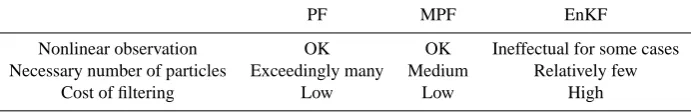
Table 4. Comparison among the algorithms for sequential data assimilation with a high-dimensional nonlinear system.
PF MPF EnKF
Nonlinear observation OK OK Ineffectual for some cases
Necessary number of particles Exceedingly many Medium Relatively few
Cost of filtering Low Low High
For cases in which the relationship between a state in the system and observed data is linear, the EnKF basically pro-vides a good estimation without a large number of particles. However, the EnKF tends to require a higher computational cost at each filtering step in applying to a high-dimensional model, because it involves many multiplications and addi-tions between matrices. In addition, even if the number of particles is taken to be small, estimates using the EnKF can be affected by spurious correlations between distant lo-cations, and thus localization on the covariance matrix (Ott et al., 2004) might be required to avoid this problem. On the other hand, a computational cost at each filtering step is not serious in the MPF, because neither iterative calculations of inverse matrices nor numerous multiplications between ma-trices are required. Therefore, for cases in which a system model does not require a great deal of computational time, the MPF may perform better than the EnKF.
Table 4 summarizes the characteristics of the algorithms of the PF, the MPF, and the EnKF. In the cases of a nonlin-ear relationship between a state and observed data, the EnKF does not necessarily work, whereas the PF or the MPF can be applied. The PF requires an exceedingly large number of particles, which imposes prohibitive computational cost at each forecast step. The MPF requires far fewer particles than the PF, although the EnKF requires fewer particles than the MPF. As for the computational cost at each filtering step, the EnKF requires a larger computational cost than the PF and the MPF. The high computational cost at each filtering step would become serious in the case that the number of assim-ilated data is large. On the other hand, the increase in the number of particles causes a high computational cost at each forecasting step, which becomes serious for the case in which a system model requires a great deal of computational time. Therefore, for the case in which only linear observations are used, the choice between the MPF and the EnKF should be made based on the considerations of the dimension of the ob-servation vector and the computational cost required by the system model.
Acknowledgements. This study was supported by the Japan
Science and Technology Agency (JST) under the Core Research for Evolutional Science and Technology (CREST) program, and partially supported by the Transdisciplinary Research Integration Center, Research Organization of Information and Systems (ROIS/TRIC) as a Function and Induction Research Project.
Edited by: O. Talagrand
Reviewed by: P. J. van Leeuwen and two other anonymous referees
References
Anderson, J. L.: A ensemble adjustment Kalman filter for data as-similation, Mon. Wea. Rev., 129, 2884–2903, 2001.
Anderson, J. L. and Anderson, S. L.: A Monte Carlo implemen-tation of the nonlinear filtering problem to produce ensemble assimilations and forecasts, Mon. Wea. Rev., 127, 2741–2758, 1999.
Burgers, G., van Leeuwen, P. J., and Evensen, G.: Analysis scheme in the ensemble Kalman filter, Mon. Wea. Rev., 126, 1719–1724, 1998.
Evensen, G.: Using the extended Kalman filter with a multilayer quasi-geostrophic model, J. Geophys. Res., 97(C11), 17 905– 17 924, 1992.
Evensen, G.: Sequential data assimilation with a nonlinear quasi-geostrophic model using Monte Carlo methods to forecast error statistics, J. Geophys. Res., 99(C5), 10 143–10 162, 1994. Evensen, G.: The ensemble Kalman filter: theoretical
formula-tion and practical implementaformula-tion, Ocean Dynam., 53, 343–367, doi:10.1007/s10236-003-0036-9, 2003.
Goldberg, D. E.: Genetic algorithms in search, optimization and machine learning, Addison-Wesley, Reading, 1989.
Gordon, N. J., Salmond, D. J., and Smith, A. F. M.: Novel approach to nonlinear/non-Gaussian Bayesian state estimation, IEE Pro-ceedings F, 140, 107–113, 1993.
Higuchi, T. and Kitagawa, G.: Knowledge discovery and self-organizing state space model, IEICE Transactions on Informa-tion and Systems, E83-D, 36–43, 2000.
H¨urzeler, M. and K¨unsch, H. R.: Monte Carlo approximations for general state space models, J. Comp. Graph. Statist., 7, 175–191, 1998.
Kitagawa, G.: Monte Carlo filtering and smoothing method for non-Gaussian nonlinear state space model, Inst. Statist. Math. Res. Memo., 1993.
Kitagawa, G.: Monte Carlo filter and smoother for non-Gaussian nonlinear state space models, J. Comp. Graph. Statist., 5, 1–25, 1996.
Kitagawa, G. and Gersch, W.: Smoothness priors analysis of time series, chap. 6, Springer-Verlag, New York, 1996.
Kivman, G. A.: Sequential parameter estimation for stochastic sys-tems, Nonlin. Process. Geophys., 10, 253–259, 2003.
Kotecha, J. H. and Djuri´c, P. M.: Gaussian particle filtering, IEEE Trans. Signal Processing, 51, 2592–2601, 2003.
Lorenz, E. N. and Emanuel, K. A.: Optimal sites for supplementary weather observations: Simulations with a small model, J. Atmos. Sci., 55, 399–414, 1998.
Musso, C., Oudjane, N., and Le Gland, F.: Improving regularized particle filters, in: Sequential Monte Carlo methods in practice, edited by Doucet, A., de Freitas, N., and Gordon, N., chap. 12, p. 247, Springer-Verlag, New York, 2001.
Nerger, L., Hiller, W., and Schr¨oter, J.: A comparison of error sub-space Kalman filters, Tellus, 57A, 715–735, 2005.
Ott, E., Hunt, B. R., Szunyogh, I., Zimin, A. V., Kostelich, E. J., Corazza, M., Kalnay, E., Patil, D. J., and Yorke, J. A.: A local ensemble Kalman filter for atmospheric data assimilation, Tellus, 56A, 415–428, 2004.
Pham, D. T., Verron, J., and Gourdeau, L.: Singular evolutive Kalman filters for data assimilation in oceanography, C. R. Acad. Sci. Ser. II, 326, 255–260, 1998a.
Pham, D. T., Verron, J., and Roubaud, M. C.: A singular evolutive extended Kalman filter for data assimilation in oceanography, J. Mar. Syst., 16, 323–340, 1998b.
van Leeuwen, P. J.: A variance-minimizing filter for large-scale ap-plications, Mon. Wea. Rev., 131, 2071–2084, 2003.