www.atmos-meas-tech.net/8/4845/2015/ doi:10.5194/amt-8-4845-2015
© Author(s) 2015. CC Attribution 3.0 License.
OMI total column ozone: extending the long-term data record
R. D. McPeters1, S. Frith2, and G. J. Labow2
1Laboratory for Atmospheres, Code 614, NASA Goddard Space Flight Center, Greenbelt, MD, USA 2Science Systems and Applications Inc., 10210 Greenbelt Rd., Lanham, MD 20706, USA
Correspondence to: R. D. McPeters ([email protected])
Received: 18 May 2015 – Published in Atmos. Meas. Tech. Discuss.: 21 July 2015 Revised: 13 October 2015 – Accepted: 26 October 2015 – Published: 19 November 2015
Abstract. The ozone data record from the Ozone Monitor-ing Instrument (OMI) onboard the NASA Earth ObservMonitor-ing System (EOS) Aura satellite has proven to be very stable over the 10-plus years of operation. The OMI total column ozone processed through the Total Ozone Mapping Spec-trometer (TOMS) ozone retrieval algorithm (version 8.5) has been compared with ground-based measurements and with ozone from a series of SBUV/2 (Solar Backscatter Ultravi-olet) instruments. Comparison with an ensemble of Brewer– Dobson sites shows an absolute offset of about 1.5 % and almost no relative trend. Comparison with a merged ozone data set (MOD) created by combining data from a series of SBUV/2 instruments again shows an offset, of about 1 %, and a relative trend of less than 0.5 % over 10 years. The offset is mostly due to the use of the old Bass–Paur ozone cross sections in the OMI retrievals rather than the Brion– Daumont–Malicet cross sections that are now recommended. The bias in the Southern Hemisphere is smaller than that in the Northern Hemisphere, 0.9 % vs. 1.5 %, for reasons that are not completely understood. When OMI was compared with the European realization of a multi-instrument ozone time series, the GTO (GOME type Total Ozone) data set, there was a small trend of about −0.85 % decade−1. Since all the comparisons of OMI relative to other ozone measuring systems show relative trends that are less than 1 % decade−1, we conclude that the OMI total column ozone data are suffi-ciently stable that they can be used in studies of ozone trends.
1 Introduction
While ozone has sometimes been referred to as a “solved problem”, it is important to continue to monitor ozone. Accu-rate measurements of altitude- and latitude-dependent ozone
trends are needed to verify the accuracy of the models that are being used to predict the expected behavior of ozone in the next 100 years (Park et al., 1999). Because climate change and ozone change turn out to be intimately related (McLin-den and Fioletov, 2011), continuing an accurate ozone record is also important for verification of the climate models.
Under NASA’s MEaSUREs program, an acronym for Making Earth System data records for Use in Research En-vironments, a long-term ozone data record was created using data from a series of SBUV and SBUV/2 (Solar Backscat-ter Ultraviolet) instruments (McPeBackscat-ters et al., 2013) covering the period from 1979 to the present. A consistent calibration was applied at the radiance level to create this time series. Data from this series of SBUV/2 instruments were combined into a single ozone time series (Frith et al., 2014), which we designate the MOD (merged ozone data) time series. Data from the Ozone Monitoring Instrument (OMI), which was launched in 2004 on the Aura spacecraft, overlap data from SBUV/2 instruments on NOAA 16, NOAA 17, NOAA 18, and NOAA 19. Since June of 2014 only the instrument on NOAA 19 continues to operate.
Data from the Ozone Mapping Profiler Suite (OMPS) nadir profiler instrument on Suomi National Polar-orbiting Partnership (NPP), which began operation in 2012, will be used to continue the MOD time series. If the OMI ozone can be shown to be a stable, well-calibrated time series, OMI ozone can be an important bridge between the SBUV/2 ozone and the OMPS ozone. Moreover, because OMI pro-vides full global coverage on a daily basis where SBUV/2 measures only along the sub-satellite track at 26◦longitude
2 The OMI ozone data record
The Ozone Monitoring Instrument (OMI) (Levelt et al., 2006) is a contribution of the Netherlands’s Agency for Aerospace Programmes (NIVR) in collaboration with the Finnish Meteorological Institute (FMI) to the NASA Aura mission. OMI is a nadir-viewing, wide-swath, ultraviolet– visible imaging spectrometer that provides daily global mea-surements of the solar radiation backscattered by the Earth’s atmosphere and surface, along with measurements of the so-lar irradiance. Unlike the heritage TOMS (Total Ozone Map-ping Spectrometer) instruments which measure ozone using six discrete wavelengths from 306 to 380 nm, OMI measures the complete spectrum from 270 to 500 nm at an average spectral resolution of 0.5 nm. Like TOMS, OMI provides complete global maps of total column ozone on a daily basis. Two distinct algorithms have been used to compute total column ozone from OMI, a TOMS-type algorithm, hereafter referred to as OMI-TOMS, and a differential optical absorp-tion spectroscopy (DOAS) algorithm (Veefkind et al., 2006). A variation of the version 8 TOMS algorithm (Bhartia, 2007) used to process data from the series of TOMS instruments has been used for the OMI-TOMS retrieval. In this paper we use the OMI-TOMS retrieval, partly because after 20 years of development it is a very robust algorithm, and also in order to maintain continuity with a TOMS data record that dates back to November 1978. Designated the v8.5 algorithm, the most significant enhancement is that the longer wavelengths measured by OMI are used to infer cloud height on a scene-by-scene basis.
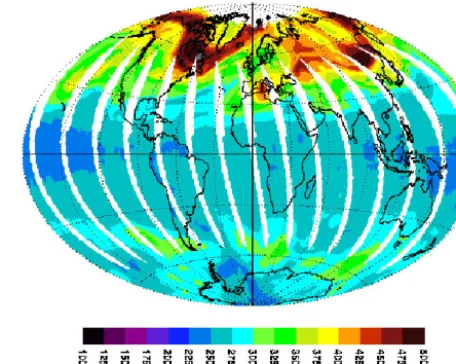
The OMI ozone data record starts in October 2004, shortly after the launch of Aura. Beginning in approximately 2008 the instrument began to experience partial blockage of its field of view as the protective film on the spacecraft began to peel. This effect known as the “row anomaly” results in the loss of data for the fields of view in the center-right part of each swath of observations. The affected data are uncor-rectable and are flagged so that they are not used in analysis. The result is small stripes of missing data each orbit (Fig. 1) for the post-2008 period. While the flagging is not perfect, comparisons in this paper will show that the residual ozone errors are small.
The stability of OMI is monitored by tracking onboard in-strument parameters (Dobber et al., 2008), by routine mea-surements of solar flux, and by tracking the stability of geo-physical parameters like average ice reflectivity in Greenland and Antarctica. All these parameters show that OMI has been a far more stable instrument than the previous TOMS instru-ments.
3 Ozone comparisons
The stability of the OMI ozone data record has been eval-uated through comparisons with ground-based observations
Figure 1. OMI gives full daily coverage except for stripes of data loss due to the row anomaly error beginning in 2008.
and with other satellite data sets. The previous analysis of the initial 2-year period of OMI data (McPeters et al., 2008) showed that the OMI-TOMS data had no evidence of drift relative to the ground network. Figure 2 compares average ozone from 76 Northern Hemisphere Brewer–Dobson sta-tions with coincident observasta-tions of ozone measured by OMI over individual stations (Labow et al., 2013). Such com-parisons have been shown capable of detecting instrument changes of a few tenths of a percent (McPeters at al., 2008). The linear fit in Fig. 2 shows that OMI has almost no drift in ozone relative to the ground observations (0.05 % decade−1). The offset of about−1.5 % is mostly caused by the use of the older Bass–Paur ozone cross sections (Bass and Paur, 1984) in the OMI retrievals rather than the newer Brion–Daumont– Malicet ozone cross sections (Brion et al., 1993; Malicet et al., 1995). While Brewer–Dobson retrievals also use Bass– Paur cross sections, analysis shows that, unlike OMI, there is little change in the Brewer–Dobson retrievals when the newer cross sections are used. This is because the ground-based in-struments use different sets of wavelengths than OMI.
2006 2008 2010 2012 2014 2016 Date
-4 -3 -2 -1 0 1
% Difference
Figure 2. A comparison of OMI ozone with average ozone from an ensemble of 76 Northern Hemisphere Dobson–Brewer stations, with linear fit also shown. Weekly mean percent difference of OMI ozone minus ground-based ozone is plotted.
total ozone with the Brewer–Dobson network showed agree-ment to within 1 % over the 30-year period of comparison (Labow et al., 2013).
Figure 3 compares ozone measured by OMI with that mea-sured by one of the instruments, the SBUV/2 on NOAA 18, which was operational and in a near-noon orbit over most of the OMI time period. (Data from the NOAA 16 instrument, for example, are noisier and sometimes not available in the 2008–2012 period as the spacecraft orbit drifted through the terminator.) The monthly zonal average ozone area weighted for the latitude zone from 60◦S to 60◦N is plotted. Because ozone is derived from measurements of backscattered sun-light, data are not always available in winter months at lati-tudes above 60◦. The lower panel in Fig. 3 shows the monthly average ozone measured by each instrument, while the up-per panel shows the up-percent difference of OMI ozone minus N18 SBUV ozone. The important point is that the relative trend between OMI and N18 is less than 0.1 % per decade. The offset of−1.1 % is again mostly caused by the fact that the Bass–Paur ozone cross sections were used for the OMI processing while the Brion–Daumont–Malicet ozone cross sections were used for the SBUV v8.6 processing. The up-coming reprocessing of OMI data using a version 9 ozone algorithm will use the new cross sections and should reduce the bias seen in Fig. 3.
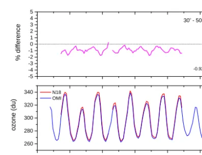
Figures 4 and 5 show similar comparisons for the southern midlatitudes (30 to 50◦S) and for the northern midlatitudes (30 to 50◦N) respectively. In each case the amplitude of the annual cycle is somewhat bigger than for the global average since annual variation in the two hemispheres largely cancels in the global average. This is reflected in the percent differ-ence plot as an annual cycle in the differdiffer-ence of about 1 %. The relative trend of OMI vs. NOAA 18 SBUV/2 is very small, no more than 0.1 % per decade when a linear fit is done for the difference plot (upper panel in each plot).
-5 -4 -3 -2 -1 0 1 2 3 4 5
2004 2006 2008 2010 2012 2014 240
260 280 300 320 340
-1.10%
% difference
60o S - 60o N
N18 OMI
ozone (du)
Year
Figure 3. The ozone time series averaged from 60◦S to 60◦N for OMI and for the SBUV/2 on NOAA 18 are shown in the bottom plot. The percent difference in the upper plot shows that OMI ozone had very little trend relative to N18 but had an average bias of
−1.1 %.
-5 -4 -3 -2 -1 0 1 2 3 4 5
2004 2006 2008 2010 2012 2014 260
280 300 320 340
-0.92%
% difference
30o
- 50o
S
N18 OMI
ozone (du)
Year
Figure 4. A similar time series albeit averaged from 30 to 50◦S shows that ozone in the Southern Hemisphere was also stable rela-tive to N18 with a seasonal dependance of about 1 %.
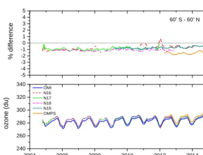
Figure 6 presents a comprehensive picture of OMI ozone relative to that from the four NOAA instruments, as well as a comparison with the initial processing of data from the OMPS nadir mapper on Suomi NPP. Comparisons of the data records from the SBUV instruments with other instru-ments are discussed in the Frith et al. (2014) validation pa-per. Here, as before, global average ozone from 60◦S to
60◦N is plotted as well as percent difference for each
in-strument. The first thing to note is the high degree of con-sistency of the four NOAA instruments. Not counting the OMPS data which have yet to be processed using a final calibration, the average trend of OMI relative to SBUV was
per--5 -4 -3 -2 -1 0 1 2 3 4 5
2004 2006 2008 2010 2012 2014 280
300 320 340 360
-1.53%
% difference
30o - 50o N
N18 OMI
ozone (du)
Year
Figure 5. A similar time series albeit averaged from 30 to 50◦N shows that ozone in the Northern Hemisphere was also stable rela-tive to N18 but had a somewhat higher bias.
-5 -4 -3 -2 -1 0 1 2 3 4 5
2004 2006 2008 2010 2012 2014 240
260 280 300 320 340
% difference
60o
S - 60o
N
OMI N16 N17 N18 N19 OMPS
ozone (du)
Year
Figure 6. The OMI ozone time series averaged over the zone 60◦S to 60◦N is compared with ozone from four SBUV/2 instruments on NOAA satellites and with the OMPS mapper on Suomi NPP.
cent per decade level, it is not possible to say whether the SBUV trend is more accurate than the OMI trend.
While Figs. 4 and 5 show that the trend of OMI relative to SBUV was nearly identical in the southern and north-ern hemispheres, notice that the bias is different in the two hemispheres. The bias at southern midlatitudes was−0.92 %, while the bias in the northern midlatitudes was −1.53 %. This is examined more closely in Fig. 7, which shows the average ozone and percent difference as a function of lati-tude for the month of June 2013. Relative to the NOAA 19 SBUV/2 ozone data, OMI is only about 0.5 % lower in the 15–60◦S region, but it is as much as 2 % lower near 60◦N. The question then is, is the source of the difference a latitude-dependent error in OMI, in NOAA 19, or both? And is the difference instrumental or algorithmic? The OMI-TOMS re-trieval uses wavelengths longer than 315 nm to derive total column ozone, while the SBUV algorithm uses wavelengths shorter than 310 nm to retrieve an ozone profile and then
inte--5 -4 -3 -2 -1 0 1 2 3 4 5
-90 -60 -30 0 30 60 90
180 220 260 300 340 380 420
% difference
OMI NPP mapper N19 SBUV/2
ozone (du)
latitude
Figure 7. Latitude dependence of OMI relative to N19 SBUV/2 and the NPP OMPS mapper for June of 2013.
grates the profile to determine total column ozone. In princi-ple the SBUV retrieval should be more accurate, particularly at high solar zenith angles. But the highest solar zenith angles in June are in the Southern Hemisphere, where the difference is only about 0.5 %.
June of 2013 was chosen for this comparison because data were also available from the NPP OMPS nadir mapper, an in-strument quite similar to OMI. While the final calibration for OMPS has yet to be determined, the algorithm used to derive total column ozone is very similar to the OMI-TOMS algo-rithm. This should help eliminate the algorithm as the source of the latitude dependence. In the Fig. 7 percent difference plot the NPP mapper (the solid blue curve) shows a latitude dependence similar to that for SBUV. This suggests (but does not prove) that there might be a small instrumental effect in OMI that leads to the observed hemispheric asymmetry.
4 Comparison with merged data sets
-5 -4 -3 -2 -1 0 1 2 3 4 5
2004 2006 2008 2010 2012 2014 240
260 280 300 320 340
% difference
60o S - 60o N
OMI MOD GTO
ozone (du)
Year
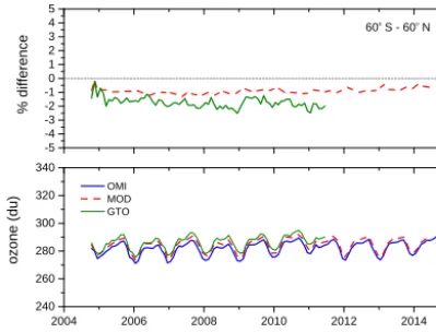
Figure 8. The MOD (merged ozone data) based on SBUV/2 instru-ments and the GTO (GOME type Total Ozone) merged ozone based on GOME instruments and SCIAMACHY are compared with OMI.
In Fig. 8 OMI ozone averaged from 60◦S to 60◦N is
com-pared with the v8.6 MOD time series based on our best-effort merger of the NASA SBUV/2 data (Frith et al., 2014) and with the GTO time series described above. The OMI bias rel-ative to GTO is a bit larger,−1.7 % vs.−1.0 % for MOD over the same time period. These results are consistent with the re-sult of comparisons shown in Chiou et al. (2014). While OMI has almost no trend relative to MOD over the 2004–2011 time period, the trend relative to GTO is−0.85 % decade−1. This of course implies that the GTO time series ozone in-creases about 0.8 % decade−1 relative to the MOD ozone. Is this significant? Given the difficulty of maintaining long-term calibration of multi-instrument data sets, 1 % decade−1 is probably the best anyone can do, and these differences are within the range of uncertainty.
5 Conclusions
OMI has proven to be one of the most stable ozone instru-ments that has been flown on a NASA satellite. Compar-ison with a network of 76 Northern Hemisphere ground-based Dobson–Brewer instruments shows very good agree-ment over a 10-year comparison period. The bias of OMI relative to other observations of about 1.5 % is due mostly to the use of the older Bass–Paur ozone cross sections.
OMI data were compared with the version 8.6 process-ing of data from SBUV/2 instruments on NOAA 16, 17, 18, and 19. For this processing the radiances for each SBUV/2 instrument were carefully analyzed and adjusted to create a consistent ozone data series suitable for trend analysis. The resulting total ozone time series agreed well with other satellite series and with the ground network. Relative to the SBUV time series OMI shows a small time dependence of
+0.45 % decade−1and an average bias of−0.9 %. One odd result that is not completely understood is that the bias of OMI relative to SBUV and to OMPS was slightly larger in
the Northern Hemisphere than in the Southern Hemisphere, by about 0.5 %.
When OMI was compared with the European realization of a multi-instrument ozone time series, the GTO data set, there was a small trend of about−0.85 % decade−1 and a slightly larger bias than for the NASA MOD data set.
Our conclusion is that OMI continues to be a high-quality ozone data set usable for trend analysis provided the later (post-2008) data are screened for row anomaly effects. The trends of OMI ozone relative to the merged data sets, MOD and GTO, were all less than 1 % decade−1, which is arguably the best anyone can do with the present instrument systems.
Data Availability
Data from Aura are easily available online from the Goddard Data and Information Services Center (DISC): http://disc.sci. gsfc.nasa.gov/Aura.
The OMI data product used here is designated OMTO3. The OMI DOAS ozone product is also available from this site.
The OMTO3 level 3 gridded ozone data are also available from the Goddard anonymous FTP account: ftp://toms.gsfc. nasa.gov. The data are in the directory pub/omi/data/ozone. Preliminary data for the NPP OMPS mapper are also available from this anonymous FTP site, in the directory pub/omps_tc/data/ozone. The v8.6 MOD data are available from http://acdb-ext.gsfc.nasa.gov/Data_services/merged.
Acknowledgements. The Dutch–Finnish-built OMI instrument is part of the NASA EOS Aura satellite payload. OMI total ozone column data were processed at NASA and jointly analyzed by the US–Dutch–Finnish science team. The version 8.6 SBUV data set was created under NASA’s MEaSUREs program for the production of multi-instrument data sets. We thank the many people who have worked over the years to understand the behavior of OMI and of the SBUV instruments in order to produce accurate ozone data products.
Edited by: V. Sofieva
References
Bass, A. M. and Paur, R. J.: The ultraviolet cross-sections of ozone. I. The measurements, in: Proc. Quadrenniel Ozone Symp., Halkidiki, Greece, 3–7 September, 1984, edited by: Zerefos, C. and Ghazi, A., Reidel, Dordecht, 606–616, 1984.
Bhartia, P. K.: Total ozone from backscattered ultraviolet measure-ments, in: Observing Systems 20 for Atmospheric Composition, L’Aquila, Italy, 20–24 September, 2004, edited by: Visconti, G., Di Carlo, P., Brune, W., Schoeberl, W., and Wahner, A., Springer, 48–63, 2007.
Chiou, E. W., Bhartia, P. K., McPeters, R. D., Loyola, D. G., Coldewey-Egbers, M., Fioletov, V. E., Van Roozendael, M., Spurr, R., Lerot, C., and Frith, S. M.: Comparison of profile total ozone from SBUV (v8.6) with GOME-type and ground-based total ozone for a 16-year period (1996 to 2011), Atmos. Meas. Tech., 7, 1681–1692, doi:10.5194/amt-7-1681-2014, 2014. Coldewey-Egbers, M., Loyola, D. G., Koukouli, M., Balis, D.,
Lambert, J.-C., Verhoelst, T., Granville, J., van Roozendael, M., Lerot, C., Spurr, R., Frith, S. M., and Zehner, C.: The GOME-type Total Ozone Essential Climate Variable (GTO-ECV) data record from the ESA Climate Change Initiative, Atmos. Meas. Tech., 8, 3923–3940, doi:10.5194/amt-8-3923-2015, 2015. Dobber, M., Kleipool, Q., Dirksen, R., Levelt, P., Jaross, G., Taylor,
S., Kelly, T., and Flynn, L.: Validation of ozone monitoring in-strument level-1b data products, J. Geophys. Res., 113, D15S06, doi:10.1029/2007JD008665, 2008.
Frith, S. M., Kramarova, N. A., Stolarski, R. S., McPeters, R. D., Bhartia, P. K., and Labow, G. J.: Recent changes in total column ozone based on the SBUV Version 8.6 merged ozone data set, J. Geophys. Res., 119, 9735–9751, doi:10.1002/2014JD021889, 2014.
Labow., G., McPeters, R., Bhartia, P. K., and Kramarova, N.: A comparison of 40 years of SBUV measurements of column ozone with data from the Dobson/Brewer network, J. Geophys. Res., 118, 7370–7378, doi:10.1002/jgrd.50503, 2013.
Lerot, C., VanRoozendael, M., Spurr, R., Coldewey-Egbers, M., Kochenova, S., vanGent, J., Koukouli, M., Balis, D., Lam-bert, J., Granville, J., and Zehner, C.: Homogenized total ozone data records from the European sensors GOME/ERS-2, SCIA-MACHY/Envisat and GOME- 2/MetOp-A, J. Geophys. Res., 119, D07302, doi:10.1002/2013JD020831, 2014.
Levelt, P. F., Hilsenrath, E., Leppelmeier, G., van den Oord, G., Bhartia, P. K., Tamminen, J., de Haan, J., and Veefkind, J.: Science Objectives of the Ozone Monitoring Instru-ment, IEEE Trans. Geosci. Remote Sens., 44, 1199–1208, doi:10.1109/TGRS.2006.872336, 2006.
Malicet, J., Daumont, D., Charbonnier, J., Parisse, C., Chakir, A., and Brion, J.: Ozone UV spectroscopy II. absorption cross-sections and temperature dependence, J. Atmos. Chem., 21, 263– 273, 1995.
McLinden, C. A. and Fioletov, V.: Quantifying stratospheric ozone trends: complications due to stratospheric cooling, Geophys. Res. Lett., 38, L03808, doi:10.1029/2010GL046012, 2011. McPeters, R. D., Kroon, M., Labow, G., Brinksma, E., Balis,
D., Petropavlovskikh, I., Veefkind, J., Bhartia, P. K., and Lev-elt, P.: Validation of the Aura Ozone Monitoring Instrument total column ozone product, J. Geophys. Res., 113, D15S14, doi:10.1029/2007JD008802, 2008.
McPeters, R. D., Bhartia, P. K., Haffner, D., Labow, G., and Flynn, L.: The version 8.6 SBUV ozone data record: an overview, J. Geophys. Res., 118, 1–8, doi:10.1002/jgrd.50597, 2013. Park, J. H., Ko, M., Jackman, C., Plumb, R., Kaye, J., and Sage,
K.: Models and Measurements Intercomparison II, edited by: Park, J., Ko, M., Jackman, C., Plumb, R., Kaye, J., and Sage, K., Hampton Virginia, NASA/TM-1999-209554, 1999. Veefkind, J. P., De Haan, J., Brinksma, E., Kroon, M., and Levelt,