Avalanches in bi-directional sandpile and burning models: a comparative study

(1)

European Geosciences Union

in Geophysics

Avalanches in bi-directional sandpile and burning models: a

comparative study

M. Gedalin1, M. Bregman1, M. Balikhin2, D. Coca2, G. Consolini3, and R. A. Treumann4

1_{Ben-Gurion University, Beer-Sheva, Israel} 2_{ACSE, University of Sheffield, Sheffield, UK}

3_{Ist. Fisica Spazio Interplanetario, Istituto Nazionale di Astrofisica, Rome, Italy} 4_{Max-Planck-Institute for Extraterrestrial Physics, Garching, Germany}

Received: 4 February 2005 – Revised: 29 March 2005 – Accepted: 5 April 2005 – Published: 29 July 2005 Part of Special Issue “Nonlinear and multiscale phenomena in space plasmas”

Abstract. We perform a statistical analysis of two

one-dimensional avalanching models: the bi-directional sandpile and the burning model (described in detail in the compan-ion paper by Gedalin et al. (2005) “Dynamics of the burn-ing model”). Such a comparison helps understand whether very limited measurements done by a remote observer may provide sufficient information to distinguish between the two physically different avalanching systems. We show that the passive phase duration reflects the avalanching nature of the system. The cluster size analysis may provide some clues. The distribution of the active phase durations shows a clear difference between the two models, reflecting the depen-dence on the internal dynamics. Deeper insight into the ac-tive phase duration distribution even provides information about the system parameters.

1 Introduction

Avalanching models and the concept of self-organized crit-icality (SOC) (Bak et al., 1987, 1988; Jensen, 1998) made their way to space physics quite a while ago (see,e.g. Lu and Hamilton, 1991; Chang, 1992; Lu, 1995; Consolini, 1997; Chapman et al., 1998; Boffetta et al., 1999; Chang, 1999; Takalo et al., 1999; Consolini and De Michelis, 2001; Kras-noselskikh et al., 2002; Valdivia, 2003; Lui, 2004, for a by far incomplete list). SOC ideas have been extensively used for the explanation of the behavior of reconnecting systems (Chang, 1999; Chapman et al., 1998; Charbonneau et al., 2001; Boffetta et al., 1999; Consolini and De Michelis, 2001; Klimas et al., 2004; Krasnoselskikh et al., 2002; Lu and Hamilton, 1991; Takalo et al., 1999; Valdivia, 2003; Urit-sky et al., 2001, 2002; Klimas et al., 2004). While attractive,

Correspondence to: M. Gedalin

([email protected])

these applications to space systems pose the serious problem of interpreting observations a remote observer makes within the context of the possible dynamical avalanching processes occurring at a place to which the observer has no direct ac-cess. Indeed, for example, localized reconnection throughout the current sheet cannot be studied directly without a net of spacecraft deployed in space which provides permanent mea-surements of the current sheet parameters. Since this does not seem possible in the nearest future, one has to rely on the observations of the consequences of the reconnection (go-ing on, as it is widely assumed), that is, e.g., auroral activ-ity, occuring far from the region where these activity factors were generated. Without firm knowledge of what happens between the generating and observation sites, one cannot es-tablish a reliable mapping of the auroral enhancements to the places in the current sheet where the cause comes from. Yet, with some assumptions one may try to explain the cur-rent sheet dynamics from the observations of auroral activ-ity. Some tentative studies in this direction have been done by Kozelov and Kozelova (2003). However, even in this case, there remains the question of whether usually performed sim-ple statistical analyses (power spectrum search, active and passive time durations, etc.) allow one to distinguish between various models thus bringing us to the ultimate objective -the understanding of -the underlying physics. Previous works on this topic (see, e.g. Kadanoff et al., 1989) evidenced that there are many different universality classes (each character-ized by its own scaling rule) of cellular automata models for avalanching systems with different microscopic rules.

(2)

734 M. Gedalin et al.: Avalanches in two models

Figures

0.5 1 1.5 2 2.5 3

x 105

0 20 40 60 80 100 120

time

number of active sites

Fig. 1.

Number of active sites as a function of time (bi-directional sandpile model).

1 2 3 4 5 6 7 8 9 10

x 104

20 40 60 80 100 120 140 160 180 200

time

site

9.94 9.945 9.95 9.955 9.96 9.965

x 104

10 20 30 40 50 60 70 80

time

site

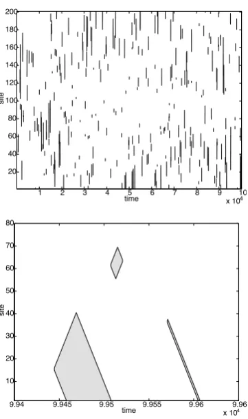
Fig. 2.

View of the sand system activity:

10

6

time steps on the left, enlarged part on the right.

Fig. 1. Number of active sites as a function of time (bi-directional

sandpile model).

0.5 1 1.5 2 2.5 3

x 105

0 20 40 60 80 100 120

time

Fig. 1.

Number of active sites as a function of time (bi-directional sandpile model).

1 2 3 4 5 6 7 8 9 10

x 104

20 40 60 80 100 120 140 160 180 200

time

site

9.94 9.945 9.95 9.955 9.96 9.965

x 104

10 20 30 40 50 60 70 80

time

site

Fig. 2.

View of the sand system activity:

10

6

11

Figures

0.5 1 1.5 2 2.5 3

x 105

0 20 40 60 80 100 120

time

Fig. 1.

Number of active sites as a function of time (bi-directional sandpile model).

1 2 3 4 5 6 7 8 9 10

x 104

20 40 60 80 100 120 140 160 180 200

time

site

9.94 9.945 9.95 9.955 9.96 9.965

x 104

10 20 30 40 50 60 70 80

time

site

Fig. 2.

View of the sand system activity:

10

6

11

Fig. 2. View of the sand system activity: 106time steps on the left, enlarged part on the right.

the avalanching system and the observer, simple statistical analysis may still appear rather inconclusive as to what kind of physics governs the system and provides the observed re-sults. Yet, certain observations may allow one to distinguish between the two systems.

2 Bi-directional sandpile model

The model is a bi-directional extension of the model de-scribed by Sanchez et al. (2002): a 2L+1 site long

sand-pile is driven randomly. Into each site Nd grains are

dropped at each times step with the probability p. If the height of (number of grains at) the sitei exceeds by more thanZc the height of at least one of the closest neighbors,

θ (N (i)−N (i+1)−Zc)+θ (N (i)−N (i−1)−Zc)>0, the site

becomes active and transfers its grains to its neighbors. The number of grains transferred to the neighbors, 2Nf, is

con-stant. If only one of the neighbors satisfies this condition it gets all the grains, if both neighbors are lower by more thanZc the transferred grains are divided equally between

the two. The grain redistribution is done numerically in two steps: first the whole array is scanned to identify the donat-ing and receivdonat-ing sites, and then the grain transfer occurs simultaneously at all relevant sites (parallel updating). Both boundaries are open, that is, N (1)=N (L)=0 is maintained throughout. In order to reduce the simulation time, we start with the distribution with a nearly critical slope and wait until the avalanching process becomes stationary. In the simula-tions the following parameters were used: L=200,Nd=10,

Zc=200, andNf=15 (similar to Sanchez et al. (2002) so that

the uni-directional results are known). The probabilitypwas used to control the avalanching activity. A typical run was several million time steps after a steady state is established.

For a remote observer, who is limited in his ability to look into the avalanching system directly, the most straightfor-ward and simple measurements would be those of the sys-tem activity. Let us assume that any giving or receiving (we shall call both active in what follows) site can be seen from a distance, so that a remote observer can reliably distinguish passive and active sites. This assumption implies, in fact, that there is a more or less well established one-to-one mapping of the avalanching region to the place where measurements are performed, like, for example, the often assumed mapping of the reconnecting current sheet in the magnetospheric tail to the auroral zone via the magnetic field lines (Klimas et al., 2004). Such a mapping requires a kind of energy transfer (for convenience we shall call it radiation) from the avalanching region to the measurement site, which means that the sys-tem should be non-conservative. In case the energy is not directly related to the grain number this non-conservation may be ignored during simulations. It should be understood, however, that a properly maintained one-to-one mapping is the essential ingredient of the model. Any non-linear prop-agation effects can, in principle, make the observed features non-resembling the true features of the avalanching system. Putting that simply, the observed radiation should reflect the features of the system we are going to analyze (e.g., cur-rent sheet) and not of some “black box” in between, other-wise there a danger of attributing the observed features to a wrong object. Assuming this does not happen, the first and most straightforward mode of measurement would be to de-tect whether the system is active (at least one of the sites is active) or passive (there are no active sites at all).

(3)

M. Gedalin et al.: Avalanches in two models 735

Table 1. Mean values for bi-directional sandpile

High state Low state

p=0.00015 p=0.00005 Mean cluster sizew¯ 12 12

Mean active phase durationTa 23 21 Mean passive phase durationTp 58 176

sites. Figures 1 and 2 show the number of active sites and the activity of the system as function of time, respectively. From both figures it is easily seen that the system is in the regime of non-weak driving and avalanche overlapping is substantial. Yet, cluster merging is negligible. The system is more active toward the edges and not active in the central part, which makes it rather similar to the directional model of Sanchez et al. (2002). Typical avalanches look as shown in the right panel. It is worth noting that a site, which was donating at some step, usually becomes receiving at the next step. If we defined as active only donating sites we would get punctuated avalanches. It also means that the length of a cluster, which does not touch a boundary, is always an even number.

In what follows we compare the cluster size distribu-tion, the active phase duration distribution and the passive phase duration distribution for the two runs with the proba-bilitiesp=0.00015 (high state) andp=0.00005 (low state). This closely corresponds to the definition of the low drive

X=pL2/Nf1 and high drivepL2/Nf&1 by Woodard et

al. (2005)1(in our case the parameterX=0.13 and 0.4, re-spectively, for the low and high states). From the observa-tion oriented point of view a more direct measure would be the percentage of time during which the system is in the ac-tive state,≈Ta/(Ta+Tp), whereTais the mean active phase

duration andTpis the mean passive state duration. This

per-centage varies from about 10% for our low state to about 30% for our high state (see below). The cluster size is the width of the connected active area fort=const. The distribution is obtained by collecting cluster sizes for all time steps.

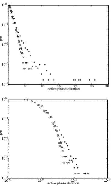
The cluster size distribution in the high state is shown in Fig. 3. The lower distribution corresponds to the odd-length clusters which are possible only when a cluster grows until it touches the edge of the sandpile (see Fig. 2). Thus, the influence of the boundaries can be clearly seen. The distribu-tion is Poisson-like with mean cluster sizew¯=12. The corre-sponding distributions of active and passive phase durations are shown in Fig. 4.

While the passive phase durations are distributed accord-ing to Poisson statistics, the active phase durations show a clear transition from the Poisson shape at low durations to a power-law behavior at larger values. The mean passive and active durations, respectively, areTp=58 andTa=23. The

1_{Woodard, R., Newman, D. E., Sanchez, R., and}

Car-reras, B. A.: Building blocks of self-organized criticality, http://arxiv.org./abs/cond-mat/0503159, 2005.

0 20 40 60 80 100 120 140 160 180 10−6

10−5

10−4 10−3

10−2

10−1

100

cluster size

pdf

Fig. 3.

Distribution of cluster sizes for the high state (bi-directional sandpile model). Log-linear scale. Upper

trend is for even-size clusters, lower is for odd-size ones. See explanation in text.

100 ₁₀1 ₁₀2 ₁₀3

10−5

10−4

10−3

10−2

10−1

100

active phase duration

pdf

0 100 200 300 400 500 600 700 10−5

10−4

10−3

10−2

10−1

100

passive phase duration

pdf

Fig. 4.

Distributions of active (left, log scale) and passive (right, log-linear scale) phase durations (bi-directional

sandpile model).

12

Fig. 3. Distribution of cluster sizes for the high state (bi-directional

sandpile model). Log-linear scale. Upper trend is for even-size clusters, lower is for odd-size ones. See explanation in text.

0 20 40 60 80 100 120 140 160 180

10−6

10−5

10−4

10−3

10−2

10−1

cluster size

pdf

Fig. 3.

Distribution of cluster sizes for the high state (bi-directional sandpile model). Log-linear scale. Upper

100 101 102 103 10−5

10−4

10−3

10−2

10−1

100

pdf

0 100 200 300 400 500 600 700 10−5

10−4

10−3

10−2

10−1

100

pdf

Fig. 4.

sandpile model).

12

0 20 40 60 80 100 120 140 160 180

10−6

10−5

10−4

10−3

10−2

10−1

100

cluster size

pdf

Fig. 3.

Distribution of cluster sizes for the high state (bi-directional sandpile model). Log-linear scale. Upper

100 ₁₀1 ₁₀2 ₁₀3

10−5

10−4

10−3

10−2

10−1 100

pdf

0 100 200 300 400 500 600 700 10−5

10−4

10−3

10−2

10−1 100

pdf

Fig. 4.

sandpile model).

Fig. 4. Distributions of active (left, log scale) and passive (right,

log-linear scale) phase durations (bi-directional sandpile model).

transition from Poisson to power-law for active phase dura-tions occurs near the mean value.

Instead of presenting separately the corresponding distri-butions for the low state we provide a comparative view, plot-ting the distributions against the normalized variables:w/w¯

for the normalized cluster size,T /Ta,p for the normalized

(4)

736 M. Gedalin et al.: Avalanches in two models

10−1 ₁₀0 ₁₀1 ₁₀2

10−5 10−4 10−3 10−2 10−1 100

pdf

0 2 4 6 8 10 12 10−5 10−4 10−3 10−2 10−1 100

pdf

Fig. 5.

Distribution of active (left) and passive (right) phase durations for high state (circles) and low state

(stars) in the bi-directional sandpile model. The durations are normalized with the mean values.

0 5 10 15 20 25 30 10−6 10−5 10−4 10−3 10−2 10−1 100 cluster size pdf

0 20 40 60 80 100 120 140 160 180 10−5 10−4 10−3 10−2 10−1 100

pdf

0 200 400 600 800 1000 1200 1400 10−5 10−4 10−3 10−2 10−1 100

pdf

Fig. 6.

Distributions of the cluster size, active phase duration, and passive phase duration for the case

p

=

0

.

0003

and

a

= 0

.

9

.

13

10−1 ₁₀0 ₁₀1 ₁₀2

10−5 10−4 10−3 10−2 10−1 100

pdf

0 2 4 6 8 10 12 10−5 10−4 10−3 10−2 10−1 100

pdf

Fig. 5.

Distribution of active (left) and passive (right) phase durations for high state (circles) and low state

0 5 10 15 20 25 30 10−6 10−5 10−4 10−3 10−2 10−1 100 cluster size pdf

0 20 40 60 80 100 120 140 160 180 10−5 10−4 10−3 10−2 10−1 100

pdf

0 200 400 600 800 1000 1200 1400 10−5 10−4 10−3 10−2 10−1 100

pdf

Fig. 6.

p

=

0

.

0003

and

a

= 0

.

9

.

Fig. 5. Distribution of active (left) and passive (right) phase

dura-tions for high state (circles) and low state (stars) in the bi-directional sandpile model. The durations are normalized with the mean values.

One can see that the cluster size is not affected by the driving strength, the active phase duration is affected only weakly, while the passive phase duration is affected substan-tially. This is in line with the understanding that driving af-fects primarily the chances of a new avalanche to start. The cluster size depends almost solely on the internal dynamics (mechanism of avalanching), as well as the avalanche dura-tion. The latter may be (relatively weakly) affected by driv-ing since input can occur durdriv-ing the avalanche development. Yet for moderate driving this effect should not be significant, and we expect that the microprocesses in the system deter-mine the avalanche length.

The active and passive phase duration distributions are shown in Fig. 5.

The power-law parts of the active phase duration distribu-tions, as well as the passive phase durations are almost iden-tical (fluctuations at large durations are due to poor statistics) for both states.

3 Burning model

This model is described in detail in the companion paper. Here we provide only a brief description. Each ofL sites is characterized by a temperature T (i). Random heat in-put q with the probability p into each site is the external driving. When a site temperature exceeds the critical value,

10−1 100 101 102

10−5

10−4

10−3

10−2

10−1

pdf

0 2 4 6 8 10 12

10−5

10−4

10−3

10−2

10−1

pdf

Fig. 5.

Distribution of active (left) and passive (right) phase durations for high state (circles) and low state

0 5 10 15 20 25 30 10−6 10−5 10−4 10−3 10−2 10−1 100 cluster size pdf

0 20 40 60 80 100 120 140 160 180 10−5 10−4 10−3 10−2 10−1 100

pdf

0 200 400 600 800 1000 1200 1400 10−5 10−4 10−3 10−2 10−1 100

pdf

Fig. 6.

p

=

0

.

0003

and

a

= 0

.

9

.

13

10−1 100 101 102

10−5 10−4 10−3 10−2 10−1 100

pdf

0 2 4 6 8 10 12

10−5 10−4 10−3 10−2 10−1 100

pdf

Fig. 5.

Distribution of active (left) and passive (right) phase durations for high state (circles) and low state

0 5 10 15 20 25 30 10−6 10−5 10−4 10−3 10−2 10−1 100 cluster size pdf

0 20 40 60 80 100 120 140 160 180 10−5 10−4 10−3 10−2 10−1 100

pdf

0 200 400 600 800 1000 1200 1400 10−5 10−4 10−3 10−2 10−1 100

pdf

Fig. 6.

p

=

0

.

0003

and

a

= 0

.

9

.

13

10−1 100 101 102

10−5 10−4 10−3 10−2 10−1 100

pdf

0 2 4 6 8 10 12

10−5 10−4 10−3 10−2 10−1 100

pdf

Fig. 5.

Distribution of active (left) and passive (right) phase durations for high state (circles) and low state

0 5 10 15 20 25 30 10−6 10−5 10−4 10−3 10−2 10−1 100 cluster size pdf

0 20 40 60 80 100 120 140 160 180 10−5 10−4 10−3 10−2 10−1 100

pdf

0 200 400 600 800 1000 1200 1400 10−5 10−4 10−3 10−2 10−1 100

pdf

Fig. 6.

p

=

0

.

0003

and

a

= 0

.

9

.

Fig. 6. Distributions of the cluster size, active phase duration, and

passive phase duration for the casep=0.0003 anda=0.9.

T (i)>Tc, the site starts to burn, releasing isotropically the

heat fluxJ=kT. The fractiona of the heat remains in the system (propagating to the neighbors), while 1−ais radiated out (lost). Burning proceeds as long asT (i)>Tl=sTc. For

the simulations below the following parameters were used:

L=400, Tc=50, s=0.3, k=3, and q=0.05Tc. Again we

study a highp=0.001 and a lowp=0.0003 state. Since this model is dissipative we have also to analyze the effects of en-ergy losses which is done varying the parametera=0.9 and

a=0.97.

shows the distributions of cluster size, active phase dura-tion, and passive phase duration for the casep=0.0003 and

(5)

M. Gedalin et al.: Avalanches in two models 737

Table 2. Mean values for burning model

Low statep=0.0003 High statep=0.001 Low statep=0.0003 High statep=0.001 Strong dissipation Strong dissipation Weak dissipation Weak dissipation

a=0.9 a=0.9 a=0.97 a=0.97

Mean cluster sizew¯ 3.4 3.4 11 12 Mean active phase durationTa 16 18 66 77 Mean passive phase durationTp 146 44 594 188

0 2 4 6 8 10 12 10−5

10−4 10−3

10−2

10−1

100

pdf

0 2 4 6 8 10 12 14 10−5

10−4 10−3

10−2

10−1

100

pdf

Fig. 7.

Comparison of active (left) and passive (right) phase duration distributions (burning model). The

durations are normalized with the corresponding mean values. Markers: stars -

p

= 0

.

0003

,

a

= 0

.

9

, circles

-p

= 0

.

001

,

a

= 0

.

9

, pluses -

p

= 0

.

0003

,

a

= 0

.

97

, and diamonds -

p

= 0

.

001

,

a

= 0

.

97

.

0 2 4 6 8 10 12 10−4

10−3

10−2

10−1

100

pdf

Fig. 8.

Comparison of the normalized distributions for the passive phase durations, sandpile stars, burning

-circles.

14

0 2 4 6 8 10 12 10−5

10−4

10−3

10−2

10−1

100

pdf

0 2 4 6 8 10 12 14 10−5

10−4

10−3

10−2

10−1

100

pdf

Fig. 7.

Comparison of active (left) and passive (right) phase duration distributions (burning model). The

p

= 0

.

0003

,

a

= 0

.

9

, circles

-p

= 0

.

001

,

a

= 0

.

9

, pluses -

p

= 0

.

0003

,

a

= 0

.

97

, and diamonds -

p

= 0

.

001

,

a

= 0

.

97

.

0 2 4 6 8 10 12 10−4

10−3

10−2

10−1

100

pdf

Fig. 8.

-circles.

Fig. 7. Comparison of active (left) and passive (right) phase

du-ration distributions (burning model). The dudu-rations are normalized with the corresponding mean values. Markers: stars−p=0.0003,

a=0.9, circles−p=0.001,a=0.9, pluses−p=0.0003,a=0.97, and diamonds−p=0.001,a=0.97.

model. The mean cluster size is w¯=3.4, the mean active phase duration isTa=16, and the mean passive phase

dura-tion isTp=146. The systems is active for about 10% of time.

Figure 7 provides the comparison for the four runs listed in Table 2.

The behavior of the mean values is similar to what we have seen in the case of the bi-directional sandpile and in agree-ment with our expectations. The passive phase duration dis-tributions are essentially the same Poisson for all runs. The active phase duration slope is steeper for stronger dissipation (which limits the avalanche propagation).

0 2 4 6 8 10 12 10−5

10−4

10−3

10−2

10−1

pdf

0 2 4 6 8 10 12 14 10−5

10−4

10−3

10−2

10−1

pdf

Fig. 7.

Comparison of active (left) and passive (right) phase duration distributions (burning model). The

p

= 0

.

0003

,

a

= 0

.

9

, circles

-p

= 0

.

001

,

a

= 0

.

9

, pluses -

p

= 0

.

0003

,

a

= 0

.

97

, and diamonds -

p

= 0

.

001

,

a

= 0

.

97

.

0 2 4 6 8 10 12 10−4

10−3

10−2

10−1

100

pdf

Fig. 8.

-circles.

14

Fig. 8. Comparison of the normalized distributions for the passive

phase durations, sandpile−stars, burning−circles.

4 Comparison and conclusions

The above results already show that there are clear dif-ferences in the remote observations of both systems. In order to make this more clear we visualize the distribu-tions of passive and active phase duradistribu-tions for both mod-els together. For this comparison we choose the low-state,

p=0.00005, bi-directional sandpile model and the weakly-driven, p=0.0003, strongly dissipative, a=0.9, burning model. For both models the system is active for about 10% of the time. The mean active and passive phase durations for the sandpile areTa=21 andTp=176. The mean active phase

duration for the burning model,Ta=11, is strongly affected

by the lower limit≈3 on the avalanche life time, so, in or-der to ensure proper visual comparison, we truncate the dis-tribution from below, excluding from the analysis the short-est avalanches (which are most probable). With this trunca-tion, the re-normalized mean values for the burning model areTa=23 andTp=145, which is pretty similar to those for

the sandpile. Thus, for the chosen parameters, both models exhibit similar levels of activity.

Figure 8 shows the passive phase distributions for both models. The plotted distributions are normalized as fol-lows: T→T /Tp, P→P /P (Tmin). The two distributions

are identical (except for long avalanches where statistics be-comes poor).

(6)

0 5 10 15 20 25 30 10−4

10−3

10−2

10−1

pdf

10−1 ₁₀0 ₁₀1 ₁₀2

10−4

10−3

10−2

10−1

pdf

Fig. 9.

Comparison of the normalized distributions for the active phase durations, sandpile stars, burning

-circles. Left panel - log-linear scale, right panel - log-log scale.

15

0 5 10 15 20 25 30 10−4

10−3

10−2

10−1

100

pdf

10−1 ₁₀0 ₁₀1 ₁₀2

10−4

10−3

10−2

10−1

100

pdf

Fig. 9.

Comparison of the normalized distributions for the active phase durations, sandpile stars, burning

-circles. Left panel - log-linear scale, right panel - log-log scale.

Fig. 9. Comparison of the normalized distributions for the active

phase durations, sandpile−stars, burning−circles. Left panel− log-linear scale, right panel−log-log scale.

distributions coincide for short avalanches, at longer values the sandpile model clearly leaves the Poisson curve toward a power-law slope.

To summarize, we have studied two one-dimensional sys-tems exhibiting avalanching behavior which could, in princi-ple, be observed in a similar way by a remote observer. We have concentrated on two systems with similar random driv-ing and similar remote observation modes. We have shown that simple direct analysis of the quiet time (passive phase duration) observations do not, in general, provide sufficient information which could be used to reliably distinguish be-tween the two systems. More sophisticated methods, like thresholding, may be useful for the analysis (Sanchez et al., 2003; Laurson and Alava, 2004; ?), but they are outside of the scope of the present consideration. On the other hand, the avalanche lengths (active phase duration) may be useful in identifying internal properties of the physical system and the underlying mechanism of the avalanches. It is worth not-ing that the exponential active phase PDFs is not expected to be unique for the burning model, and we do not claim that the proposed burning model is the most applicable but suggest it as a plausible possibility. Our analysis should be rather con-sidered as a starting point for further studies of observable features of avalanching systems in the context of measure-ments made by a remote observer, in particular, for the

prob-limited data.

Acknowledgements. This work has been performed within the

framework of the “Observable features of avalanching systems” ISSI Science Team.

Edited by: N. Watkins

Reviewed by: Z. Voros and another referee

References

Bak, P., Tang, C., and Wiesenfeld, K.: Selforganized criticality -An explanation of 1/f noise, Phys. Rev. Lett., 59, 381–384, 1987.

Bak, P., Tang, C., and Wiesenfeld, K.: Self-organized criticality, Phys. Rev. A, 38, 364–374, 1988.

Boffetta, G., Carbone, V., Giuliani, P., Veltri, P., and Vulpiani, A.: Power laws in solar flares: Self-organized criticality or turbu-lence? Phys. Rev. Lett., 83, 4662–4665, 1999.

Chang, T.: Low-dimensional behavior and symmetry breaking of stochastic systems near criticality - Can these effects be observed in space and in the laboratory?, IEEE Transactions on Plasma Science, 20, 691–694, 1992.

Chang, T.: Self-organized criticality, multi-fractal spectra, sporadic localized reconnections and intermittent turbulence in the mag-netotail, Phys. Plasmas, 6, 4137–4145, 1999.

Chapman, S.C., Watkins, N.W., Dendy, R.O., Helander, P., and Rowlands, G.: A simple avalanche model as an analogue of for magnetospheric activity, Geophys. Res. Lett., 25, 2397–2400, 1998.

Charbonneau, P., McIntosh, S. W., Liu, H.-L., and Bogdan, T. J.: Avalanche models for solar flares (Invited Review), Solar Physics, 203, 321–353, 2001.

Consolini, G.: Sandpile cellular automata and the magnetospheric dynamics, in: Proc. of Cosmic Physics in the Year 2000, 58, 123–126, (Eds.) Aiello, S., Iucci, N., Sironi, G., Treves, A., and Villante, U., SIF, Bologna, Italy, 1997.

Consolini, G. and De Michelis, P.: A revised forest-fire cellular au-tomaton for the nonlinear dynamics of the Earth’s magnetotail, JASTP, 63, 1371–1377, 2001.

Jensen, H. J.: Self-Organized Criticality : Emergent Complex Be-havior in Physical and Biological Systems, Cambridge Univer-sity Press, 1998.

Kadanoff, L. P., Nagel, S. R., Wu, L., and Zhou, S.-M.: Scaling and universality in avalanches, Physical Review A, 39, 6524–6537, 1989.

Klimas, A. J., Uritsky, V. M., Vassiliadis, D., and Baker, D. N.: Re-connection and scale-free avalanching in a driven current-sheet model, J. Geophys. Res., 109, 2218–2231, 2004.

Kozelov, B. V. and Kozelova, T. V.: Cellular automata model of magnetospheric-ionospheric coupling, Ann. Geophys., 21, 1931–1938, 2003,

SRef-ID: 1432-0576/ag/2003-21-1931.

Krasnoselskikh, V., Podladchikova, O., Lefebvre, B., and Vilmer, N.: Quiet Sun coronal heating: A statistical model, Astron. As-trophys., 382, 699–712, 2002.

Laurson, L. and Alava, M. J.: Local waiting times in critical sys-tems, Eur. Phys. J. B, 42, 407–414, 2004.

(7)

Lu, E., and Hamilton, R. J.: Avalanches and the distribution of solar flares, Astrophys. J., 380(L89), 1991.

Lui, A. T. Y.: Testing the hypothesis of the Earth’s magnetosphere behaving like an avalanching system, Nonlin. Processes Geo-phys., 11, 701–707, 2004,

SRef-ID: 1607-7946/npg/2004-11-701.

Sanchez, R., Newman, D. E., and Carreras, B. A.: Waiting-Time Statistics of Self-Organized-Criticality Systems, Phys. Rev. Lett., 88, 8302–8305, 2002.

Sanchez, R. van Milligen, B. Ph., Newman, D. E., and Carreras, B. A.: Quiet-Time Statistics of Electrostatic Turbulent Fluxes from the JET Tokamak and the W7-AS and TJ-II Stellara, Phys. Rev. Lett., 90, 5005–5008, 2003.

Takalo, J., Timonen, J., Klimas, A. J., Valdivia, J. A., and Vas-siliadis, D.: A coupled-map model for the magnetotail current sheet, Geophys. Res. Lett., 26, 2913–2916, 1999.

Valdivia,J. A., Klimas, A., Vassiliadis, D., Uritsky, V., Takalo, J.: Self-organization in a current sheet model, Sp. Sci. Rev., 107, 515–522, 2003.

Uritsky, V., Pudovkin, M., and Steen, A.: Geomagnetic sub-storms as perturbed self-organized critical dynamics of the mag-netosphere, Journal of Atmospheric and Terrestrial Physics, 63, 1415–1424, 2001.