Comparing transient, accelerated, and equilibrium simulations of the last 30 000 years with the GENIE-1 model

(1)

of the Past

Comparing transient, accelerated, and equilibrium simulations of

the last 30 000 years with the GENIE-1 model

D. J. Lunt1, M. S. Williamson2,3,*, P. J. Valdes1, T. M. Lenton2,3, and R. Marsh4

1_{Bristol Research Initiative for the Dynamic Global Environment (BRIDGE), School of Geographical Sciences, University of}

Bristol, Bristol, UK

2_{School of Environmental Sciences, University of East Anglia, UK} 3_{Tyndall Centre, UK}

4_{National Oceanography Centre, University of Southampton, Southhampton, UK} *_{now at: Quantum Information Group, University of Leeds, Leeds, UK}

Received: 3 May 2006 – Published in Clim. Past Discuss.: 14 June 2006

Revised: 20 November 2006 – Accepted: 23 November 2006 – Published: 28 November 2006

Abstract. We examine several aspects of the

ocean-atmosphere system over the last 30 000 years, by carrying out simulations with prescribed ice sheets, atmospheric CO2

concentration, and orbital parameters. We use the GENIE-1 model with a frictional geostrophic ocean, dynamic sea ice, an energy balance atmosphere, and a land-surface scheme with fixed vegetation. A transient simulation, with bound-ary conditions derived from ice-core records and ice sheet reconstructions, is compared with equilibrium snapshot sim-ulations, including the Last Glacial Maximum (21 000 years before present; 21 kyrBP), mid-Holocene (6 kyrBP) and pre-industrial. The equilibrium snapshot simulations are all very similar to their corresponding time period in the transient simulation, indicating that over the last 30 000 years, the model’s ocean-atmosphere system is close to equilibrium with its boundary conditions. However, our simulations ne-glect the transfer of fresh water from and to the ocean, result-ing from the growth and decay of ice sheets, which would, in reality, lead to greater disequilibrium. Additionally, the GENIE-1 model exhibits a rather limited response in terms of its Atlantic Meridional Overturning Circulation (AMOC) over the 30 000 years; a more sensitive AMOC would also be likely to lead to greater disequilibrium. We investigate the method of accelerating the boundary conditions of a transient simulation and find that the Southern Ocean is the region most affected by the acceleration. The Northern Hemisphere, even with a factor of 10 acceleration, is relatively unaffected. The results are robust to changes to several tunable param-eters in the model. They also hold when a higher vertical resolution is used in the ocean.

Correspondence to: D. J. Lunt

(d.j.lunt@bristol.ac.uk)

1 Introduction

General Circulation Models (GCMs) have for many years been used to simulate paleoclimates. Typically, ‘snapshot’ equilibrium simulations of selected time-periods are car-ried out, where the boundary conditions do not vary with time. Examples include the PMIP-1 project (Joussaume and Taylor, 1995), which employed Atmospheric GCMs (AGCMs) with fixed sea surface temperatures (SSTs) or slab-oceans, and the PMIP-2 project (http://www-lsce.cea.fr/ pmip2), which employed fully coupled Atmosphere-Ocean and Atmosphere-Ocean-Vegetation GCMs. This simplifi-cation is due to the computational expense of carrying out multi-millennial transient simulations. For pragmatic rea-sons, these equilibrium simulations are usually initialised with some ocean and atmospheric state, typically from a previous simulation of another time-period (such as present-day). They are then “spun-up” for some period to allow the system to come close to equilibrium with the boundary con-ditions. At the end of the spin-up, the model is run for a further period, typically decades, to extract monthly and an-nual mean climatologies. These modelled climatologies can then be compared to paleo-proxies of the snapshot being con-sidered, for example SST data (e.g. de Vernal et al., 2005), or terrestrial temperature data (e.g. Jost et al., 2005). The de-gree of ade-greement between the model and data can be used as a measure of the accuracy and validity of the climate model, and of its ability to simulate future climates.

(2)

Table 1. A selection of GENIE-1 parameter sets. “Default” is used for the majority of the simulations, except for in Sect. 3.3, where

“Traceable”, “Low-diffusion”, and “Half-flux” are used. “Subjective” is shown for information - it is not used in this study but is used in Lenton et al. (2006). “Default” and “Low-diffusion” differ only inκv. “Default” and “Half-flux” differ only inFa. “Default” and

“Subjective” differ only inkT andτpptn. For definitons of the parameters, see Edwards and Marsh (2005).

Parameter Notation Value Units

“Default” “Traceable” “Low-diffusion” “Half-flux” “Subjective”

Ocean

Isopyc. diff. κh 2000 4126 2000 2000 2000 m2s−1

Diapyc. diff. κv 1×10−4 1.81×10−5 1.81×10−5 1×10−4 1×10−4 m2s−1

Friction λ 2.5 3.43 2.5 2.5 2.5 days−1

Wind-scale W 2 1.67 2 2 2 –

Atmosphere

T diff. amp kT 3.8×106 3.75×106 3.8×106 3.8×106 3.2×106 m2s−1

T diff. width ld 1 1.31 1 1 1 Radian

T diff. slope sd 0.1 0.07 0.1 0.1 0.1 –

qdiff. κq 1×106 1.75×106 1×106 1×106 1×106 m2s−1

T adv. coeff. βT 0 0.06 0 0 0 –

qadv. coeff. βq 0.4 0.14 0.4 0.4 0.4 –

FWF adjust. Fa 0.32 0.28 0.32 0.16 0.32 Sv

RH threshold rmax 0.85 0.85 0.85 0.85 0.85 –

P timescale τpptn 3.65 3.65 3.65 3.65 4.00 days

Sea ice

Sea ice diff. κhi 2000 6249 2000 2000 2000 m2s−1

In order to overcome model speed limitations, some pre-vious workers have employed an “acceleration” technique for transient paleo simulations, in which the boundary con-ditions are accelerated by some factor, to compress the simu-lation. Jackson and Broccoli (2003) used an AGCM coupled to a slab ocean to simulate 165 000 years of climate, acceler-ated by a factor of 30; Lorenz and Lohmann (2004) used an AOGCM to simulate 7000 years of climate, accelerated by factors of 10 and 100. We estimate the error this introduces in an AOGCM by carrying out an ensemble of transient sim-ulations with different acceleration factors, and comparing them to non-accelerated transient simulations.

The tool we use in this paper is GENIE-1 [Grid ENabled Integrated Earth system model, http://www.genie.ac.uk], an Earth system Model of Intermediate Complexity (EMIC). We examine only those aspects of the model results which we believe will be reproduced by a full-complexity GCM. These are typical timescales and global, large-region, and annual mean climatic variables which are typically well-reproduced by EMICs, such as surface temperature and sea ice extent.

2 Model and methods

GENIE-1 is an EMIC which features the following cou-pled components: a three dimensional frictional geostrophic ocean (Edwards and Marsh, 2005), a two dimensional energy moisture balance atmosphere (Edwards and Marsh, 2005;

Weaver et al., 2001; Fanning and Weaver, 1996), dynamic and thermodynamic sea ice (Edwards and Marsh, 2005; Semtner, 1976; Hibler, 1979), and a land surface physics and terrestrial carbon cycle model (Williamson et al., 2006). The model is on an equal surface area grid consisting of an ar-ray of 36 gridboxes in longitude and 36 gridboxes in lati-tude. The ocean component incorporates eddy-induced and isopycnal mixing following Griffies (1998), and has 8 equal log(z)vertical levels. In order to maintain significant North Atlantic deep water formation in a standard simulation (Ed-wards and Marsh, 2005), there is a constant surface moisture flux correction which transports fresh water from the Atlantic to the Pacific in three zonal bands, totaling 0.32 Sv (variable

Fa in Table 1; see Fig. 1 of Marsh et al., 2004). The model

(3)

30 27 24 21 18 15 12 9 6 3 0 180

200 220 240 260 280 300

Atmospheric CO2 concentration , 30kyrB − 0kyrBP

kyrBP

ppmv

30 27 24 21 18 15 12 9 6 3 0

−10 0 10 20 30 40 50 60

Ice volume relative to pre−industrial , 30kyrB − 0kyrBP

kyrBP

10

6 km

3

Peltier reconstruction (21 − 0 kyrBP) Our reconstruction (30 − 0 kyrBP) Arnold reconstruction (30 kyrBP)

Fig. 1. Time-evolution of boundary conditions over the 30 kyr simulated. (a) Atmospheric CO₂concentration [ppmv], (b) Global mean orography [m], showing our reconstruction, and that of (Peltier, 1994) and (Arnold et al., 2002) for comparison.

are ill-constrained by direct observations. For the majority of the simulations described in this paper, we use a “Default” parameter set, which was arrived at by a rather ad-hoc tuning exercise of a few key variables (not shown). It is similar to the “Subjective” parameter set used by Lenton et al. (2006). In Sect. 3.3, we test the sensitivity of the results to the choice of parameter set. The key model tunable parameters used or discussed in this paper are summarised in Table 1. We use the version of the GENIE-1 model available on the GENIE Concurrent Versions System (CVS) repository at 01:00 GMT on 1st July 2006. The boundary condition and configuration files used in this paper are also archived on the CVS reposi-tory, and are available from the lead author on request. 2.1 Boundary conditions

In order to carry out transient or equilibrium simulations of the past 30 000 years, GENIE-1 requires orbital parameters (eccentricity, obliquity, and precession), an atmospheric CO2

concentration, and 2-D fields of orography and ice sheet frac-tion.

For the orbital parameters we use the data of Berger (1978). To construct the CO2record, we initially use the

Vos-tok ice-core data of Petit et al. (1999), linearly interpolated to give one value every 1000 years. We then add anomalies calculated from the Dome C ice-core data of Monnin et al. (2004) to the lower-resolution Vostok record. The resulting record, shown in Fig. 1a, has a resolution of approximately 120 years over the period 21 kyrBP to pre-industrial, where the record from Dome C exists, and reverts to the low

reso-lution record over the period 30 kyrBP to 21 kyrBP, which is out of the range of the Monnin et al. (2004) Dome C data. All timeseries are further linearly interpolated internally within the model onto its 2-day time-step.

(4)

Fig. 2. Annual mean surface temperature in (a) our industrial simulation, and (b) our industrial simulation minus a HadSM3

pre-industrial simulation. Units are◦C.

However, allowing the land-sea mask to vary in time would result in sudden changes to the boundary conditions in the middle of a transient simulation, because the land-sea mask is constrained to be binary in this model. Due to the rela-tively large size of the gridboxes, this would result in signif-icant anomalous transient behaviour following any switches between land and ocean, which may be mistaken for a real transient response to the varying boundary conditions. This problem is likely to affect any low resolution model in which the land-sea mask is constrained to be binary. Finally, be-cause theδ18O record is actually influenced by both temper-ature and global ice volume, as well as local effects, it is likely that if anything, the high-frequency variability in our ice sheet reconstruction is too high. However, we ensure that every 1 kyr between 21 kyrBP and 0 kyrBP, our time-varying reconstruction matches that of Peltier (1994). In the context of this paper, it is better to overestimate the high-frequency variability than to underestimate it, because both the error in carrying out equilibrium simulations compared to transient simulations, and the error in carrying out accelerated sim-ulations compared to non-accelerated simsim-ulations, is likely to be underestimated if the high-frequency variability in the forcing boundary conditions is too small.

2.2 Simulations

Initially, we undertake equilibrium snapshot simulations every 3 kyr, beginning with Marine Isotope Stage III (MIS3, 30 kyrBP) and including the Last Glacial Maximum (LGM, 21 kyrBP), the mid-Holocene (6 kyrBP), and the pre-industrial (corresponding to approximately 1860 AD). The LGM and mid-Holocene have traditionally been the time pe-riods studied in paleoclimate modelling studies (e.g. Hewitt et al., 2001; Jost et al., 2005; Texier et al., 2000). All the

equilibrium simulations discussed in this paper are initialised from a 20◦_{C isothermal and stationary ocean.}

We then carry out a 30 kyr transient simulation, initialised from the end-point of the MIS3 equilibrium simulation, and compare this with the equilibrium simulations. This is fol-lowed by a series of transient 30 kyr simulations in which we accelerate the boundary conditions by factors of 2, 5, and 10. Finally, we test the robustness of the results to several key variables by repeating the simulations, first with three addi-tional parameter sets, and then with a greater vertical resolu-tion.

3 Results

3.1 Equilibrium simulations

We first compare our pre-industrial, LGM, and mid-Holocene equilibrium simulations with slab-ocean HadSM3 simulations carried out using similar orbital, ice sheet, and greenhouse gas boundary conditions (Joos et al., 2004; Ka-plan et al., 2002). HadSM3 has a fully dynamic primitive equation atmosphere, and is generally more complex than GENIE-1. Although a slab ocean model does not repre-sent changes to ocean circulation, the large scale patterns of change from these simulations compare well with fully cou-pled simulations of the LGM and mid-Holocene, and with available surface observations.

(5)

Fig. 3. Annual mean sea ice fraction in (a) our pre-industrial simulation, and (b) a pre-industrial HadSM3 simulation.

Latitude [°N]

Depth [km]

pre−industrial Atlantic MOC [Sv]

−30 0 30 60 90

−5 −4 −3 −2 −1 0

−6 −3 0 3 6 9 12 15 18 21

Latitude [°N]

Depth [km]

pre−indutrial Atlantic MOC HadCM3 [Sv]

−30 0 30 60 90

−5 −4 −3 −2 −1 0

−6 −3 0 3 6 9 12 15 18 21

Fig. 4. Annual mean Atlantic Meridional Overturning Circulation (AMOC), in (a) our pre-industrial equilibrium simulation, and (b) a

pre-industrial HadCM3 simulation. Units are Sv.

sea ice albedo feedback. Figure 3 shows the annual mean sea ice fraction from our GENIE-1 pre-industrial simulation, and from HadSM3. It can be seen that this version of GENIE-1 underestimates the sea ice fraction over the Arctic Ocean, and the sea ice extent over the Antarctic Ocean. In addition, although the Antarctic sea ice is persistent throughout the year, the Arctic sea ice completely melts for about 45 days in late boreal summer. This is clearly related to, and further enhances, the warm-pole bias. Finally, in terms of evalua-tion of our pre-industrial simulaevalua-tion, we compare the Atlantic meridional overturning circulation (AMOC) to that from a pre-industrial simulation carried out using a fully coupled

(6)

Fig. 5. (a, b) Annual mean surface temperature relative to pre-industrial in (a) our LGM equilibrium simulation, and (b) an LGM HadSM3

simulation. Units are◦C. Note the non-linear colour scale. (c,d) Annual mean sea ice fraction in (c) our LGM equilibrium simulation, and (d) an LGM HadSM3 simulation.

We now move on to examine our equilibrium paleo sim-ulations. Figure 5a shows the surface temperature anomaly, relative to pre-industrial, in our LGM simulation, and Fig. 5b shows the equivalent HadSM3 anomaly. The LGM anoma-lies are fairly similar in the two models. The largest absolute difference between the two models is over the Fennoscan-dian ice sheet, where our model underestimates the temper-ature change relative to the HadSM3 model. This is because we have constrained the land-sea mask in our model to re-main constant (that of pre-industrial) for reasons discussed in Sect. 2. In the original reconstruction (Peltier, 1994), and in the HadSM3 simulation, a large fraction of the LGM Fennoscandian ice sheet is over regions which are ocean at the pre-industrial. This means that we have underestimated

(7)

Latitude [°N]

Depth [km]

LGM Atlantic MOC [Sv]

−30 0 30 60 90

−5 −4 −3 −2 −1 0

−6 −3 0 3 6 9 12 15 18 21

Latitude [°N]

Depth [km]

LGM − pre−industrial Atlantic MOC [Sv]

−30 0 30 60 90

−5 −4 −3 −2 −1 0

−6 −4 −2 0 2 4 6

Fig. 6. Annual mean Atlantic Meridional Overturning Circulation (AMOC), (a) in our LGM equilibrium simulation, and (b) our difference

LGM minus pre-industrial. Units are Sv.

Fig. 7. Annual mean surface temperature relative to pre-industrial in (a) our mid-Holocene equilibrium simulation, and (b) a mid-Holocene

HadSM3 simulation. Units are◦C.

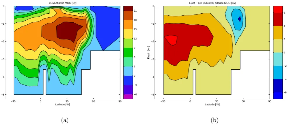
This may be related to the fact that the HadSM3 is not sim-ulating ocean circulation changes relative to modern. The LGM sea ice extent in GENIE-1 is, however, in generally good agreement with that in HadSM3. One final diagnostic of our LGM equilibrium simulations is the modelled AMOC. This is shown in Fig. 6, along with the anomaly relative to pre-industrial. The LGM circulation has the same character-istics as pre-industrial, including the lack of Antarctic bottom water penetrating into the Atlantic sector. The positive over-turning cell is in general more vigorous, and deeper, than pre-industrial. This is in contradiction to some modelling

studies, which suggest a shallowing and weakening of the in-termediate waters at the LGM; however, this is not seen in all models and there is still some degree of uncertainty about the state of the thermohaline circulation at the LGM (e.g. Weber et al., 2006; Wunsch , 2003). The positive overturning cell does not extend as far north as at pre-industrial, due to the greater extent of LGM sea ice, which forces the regions of North Atlantic deep water formation further south.

(8)

30 27 24 21 18 15 12 9 6 3 0 9

9.5 10 10.5 11 11.5 12 12.5 13 13.5

Ocean surface temp., 30kyrB − 0kyrBP

kyrBP

Temp [oC]

Control (no acceleration) x2

x5 x10

Equilibrium Simulations

30 27 24 21 18 15 12 9 6 3 0

−0.5 0 0.5 1 1.5

Global mean deep ocean temperature, 30kyrB − 0kyrBP

kyrBP

Temp [oC]

x5 x10

30 27 24 21 18 15 12 9 6 3 0

0.05 0.06 0.07 0.08 0.09 0.1 0.11 0.12 0.13

Global mean seaice fraction, 30kyrB − 0kyrBP

kyrBP

fraction

x5 x10

30 27 24 21 18 15 12 9 6 3 0

20 20.5 21 21.5 22 22.5 23 23.5 24 24.5 25

Max Atlantic overturning, 30kyrB − 0kyrBP

kyrBP

Overturning [Sv]

x5 x10

Fig. 8. (a) Temporal evolution of global-annual average ocean-surface temperature (◦C) in an ensemble of 30 kyr transient simulations. The colours represent different boundary-condition acceleration factors. The circles represent equilibrium simulations every 3 kyr. (b) shows the same but for the deep ocean temperature (approximately 5 km). Note the difference in scale between the two plots. (c) shows the same but for the sea ice fraction. (d) shows the same but for the maximum strength of the Atlantic meridional overtuning circulation (AMOC).

mid-Holocene simulations, HadSM3 exhibits significant cooling in the tropics, particularly over Saharan Africa and South Asia. The reason for this cooling is an intensification of the African and Asian monsoons, which results in greater latent cooling due to availability of soil-moisture and less in-solation due to increased cloudiness (Texier et al., 2000). The change in these regions is much weaker in our model. This is

(9)

mid-Holocene (0.4◦_{C) than at the LGM (2.9}◦_C).

In summary, the first-order response of our model to large-scale boundary-condition changes such as orography and ice sheets is in good agreement with that from a model with a dynamical atmosphere. However, our model does not simu-late more complex or localised changes such as those resimu-lated to atmospheric circulation, cloud-cover, or precipitation. 3.2 Transient simulations

Here, we present and discuss our “Default” 30 kyr transient simulation, which is initialised at the end of the MIS3 equi-librium simulation.

Figure 8a shows the global mean surface ocean tempera-ture evolution in the transient simulation (in regions of sea ice this is the temperature of the ice surface). It has a form broadly similar to the prescribed CO2 evolution, including

a minimum at 18 kyrBP. The figure also shows a compari-son of the 30 kyr transient simulation with the equilibrium simulations. It can be seen that the transient simulation is nearly always close to equilibrium (the largest deviation be-ing 24 kyrBP, which occurs just after a sharp change in ice sheet fraction). In particular, the LGM, mid-Holocene and pre-industrial are all very close to equilibrium. This is good news for model-data comparisons, such as in the PMIP2 project, where the model is calculating an equilibrium so-lution.

Figure 8a additionally shows the surface temperature evo-lution in 3 accelerated simulations, all of which are initialised at the end of the MIS3 equilibrium simulation. As expected, the greater the acceleration, the greater the error relative to the non-accelerated simulation. The accelerated simulations behave in a damped fashion relative to the non-accelerated simulation, with a decrease in magnitude of temporal tem-perature gradient, but no corresponding phase-lag. The max-imum error in global-annual mean surface temperature oc-curs in the×10 simulation, at about 11 kyrBP. There is a secondary maximum in error at about 23 kyrBP. Both these occur after and during periods of relatively rapid change in the boundary conditions, in particular the ongoing deglacia-tion between 15 kyrBP and 9 kyrBP and the sharp increase in land-ice fraction between 24 and 23 kyrBP.

Figure 8b shows the deep ocean temperatures at approx-imately 5 km depth. The temperature evolution of the deep ocean is very similar in form to that of the surface. This is not surprising given that the timescales involved are long enough for the significant surface forcing to be communicated to the deep ocean. Additionally, the changes to ocean circulation, which are a possible mechanism for a non-linear response to the surface forcing, are relatively small. The figure also illustrates the longer response time of the deep ocean rela-tive to the surface, resulting in a smoother response to the changing boundary conditions. However, there appears to be no phase-lag relative to the upper ocean, and the minimum deep-ocean temperature is also at 18 kyrBP. It also shows the

correspondingly larger relative error and significant phase lag that the acceleration technique introduces in the deep ocean. However, the transient simulation is still relatively close to equilibrium during the 30 kyr, except in the first part of the deglaciation at 15 and 12 kyrBP (even here though, the dis-equilibrium is only of the order 0.3◦C in the global annual mean).

Figure 8c shows the temporal evolution of sea ice area over the same period, again with the equilibrium and accelerated simulations also shown. It is striking how linear the rela-tionship is between sea ice fraction and temperature. As for temperature, the transient simulation is very close to equi-librium for the majority of the 30 000 years. However, the acceleration appears to have a slightly greater relative effect on sea ice than on air temperature, and there is almost a 10% difference in sea ice area between the non-accelerated and the×10 simulation at the time of the LGM. Finally, Fig. 8d shows a diagnostic for the temporal evolution of ocean cir-culation. The variable plotted is the maximum value of the AMOC below the mixed layer, i.e. the pre-industrial value is the the maximum value below the mixed layer from Fig. 4a. In the broadest terms, this shows that the AMOC is in an “on” state throughout the 30 000 years. There is a sharp de-crease around 9 kyrBP, but it is not large enough to be consid-ered a transition to a different state. Despite the relative in-sensitivity of the AMOC to the forcing boundary conditions (±7%), it displays a more non-linear response than the tem-perature or sea ice. For example, the sharp decrease around 9 kyrBP occurs when there is only a relatively small change in the prescribed ice sheet extent. We carry out a further ex-periment (not shown) to investigate this variability in more detail. In this, we do not use the Vostok δ18O record or the Dome C CO2 record to introduce high-frequency

vari-ability into the forcing boundary conditions, but use only the Vostok and Peltier records at a 1 kyr resolution. In this simulation, the response of the AMOC is much smoother. This shows that the high frequency variability seen in Fig. 8d is not generated internally, but is a non-linear response to the time-varying boundary conditions. The exception is be-tween 24 kyrBP and 21 kyrBP, where both the high- and low-frequency simulations show some high-low-frequency variabil-ity. This is most likely a manifestation of a self sustained oscillation caused by sea ice/ocean feedback in the Southern Ocean, which is also found under pre-industrial conditions in certain regions of parameter space. The effect of acceler-ation on the evolution of the AMOC appears to be relatively low, although this is unlikely to have been the case if we had simulated a significant change in the state of the circula-tion in the non-accelerated simulacircula-tion. The sensitivity of the AMOC response to the moisture flux correction is discussed in Sect. 3.3.

(10)

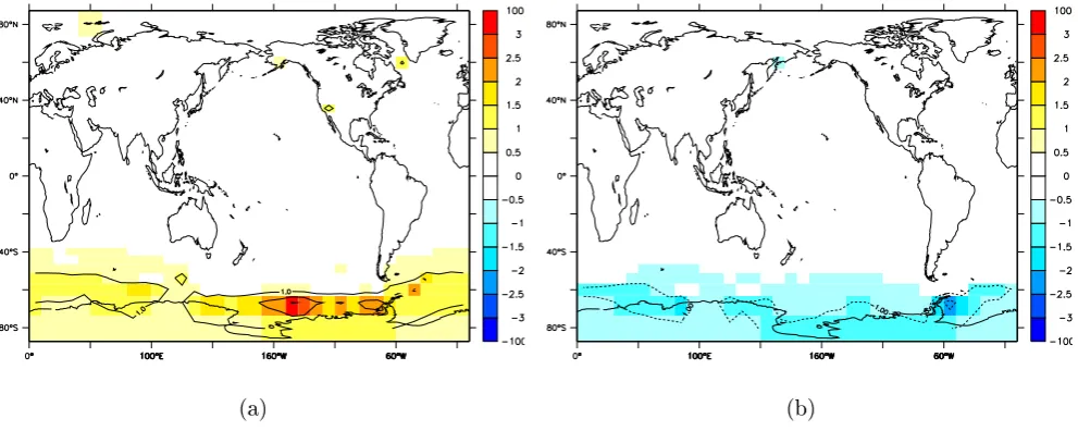
Fig. 9. Annual mean surface temperature in the×10 accelerated 30 kyr simulation, relative to the non-accelerated simulation, at (a) the LGM and (b) the mid-Holocene. Units are◦C.

temperature difference in the×10 simulation relative to the non-accelerated simulation, at the LGM and mid-Holocene. It appears that Southern Ocean is producing the damping in the system in the accelerated simulations. In this region, the local surface temperature errors are of the order of 1 or 2◦C, being too warm during the cooling LGM and too cold dur-ing the warmdur-ing mid-Holocene. This is the region with the greatest thermal inertia, due to the deep mixed-layer, and it reflects the slowly varying temperature of the deep ocean. Consequently, Antarctica also has a significant temperature error in the accelerated simulations. This effect is amplified by the sea ice-albedo feedback; for example, the accelerated simulation has too little Southern Ocean sea ice at the LGM relative to the non-accelerated simulation. In contrast, the surface temperature in the Northern Hemisphere is very well simulated in the accelerated simulations.

3.3 Sensitivity studies

In this section, we assess the sensitivity of our results to the parameter set and the ocean model vertical resolution we have used.

The simulations described so far all use the ‘Default’ pa-rameter set (shown in Table 1 along with the other papa-rameter sets discussed in this section), and 8 vertical levels. An alter-native parameter set is the “Traceable” set, found in an ob-jective tuning exercise initially carried out by Hargreaves et al. (2004) using the ensemble Kalman filter, and used in the study of Lenton et al. (2006). This was tuned to minimise the error in ocean temperature, ocean salinity, atmospheric sur-face temperature and atmospheric specific humidity, relative to modern observations. However, the exercise was carried out with a previous version of the model which contained

a simplified representation of the land surface. A further possible set is the “Low-diffusion” set. This is the same as the “Default” set except that we decrease the diapycnal dif-fusivity, κv, in the ocean from 1×10−4 to 1.81×10−5 (the

same value as in the “Traceable” set). Seeing as the typical timescale in the ocean is determined byD2/κv, whereDis

the depth of the ocean, we would expect the “Low-diffusion” set to have a typical timescale about 5 times as long as the “Default” set. A further parameter set is the “Half-flux” set. In this, the magnitude of the moisture flux correction, de-scribed in Sect. 2, is halved (variableFa in Table 1). This

simulation is carried out to test whether the relatively insen-sitive response of the AMOC is linked to the flux correction. In addition to the sensitivity to the parameter set, we also test the sensitivity to the vertical resolution of the ocean model, by carrying out a simulation, “High-resolution”, with 16 ver-tical levels in place of the usual 8.

(11)

30 27 24 21 18 15 12 9 6 3 0 8

9 10 11 12 13

Ocean surface temp. (Default parameter set)

kyrBP

Temp [oC]

x5 x10 Equilibrium Simulations

30 27 24 21 18 15 12 9 6 3 0

8 9 10 11 12 13

Ocean surface temp. (Traceable parameter set)

kyrBP

Temp [oC]

30 27 24 21 18 15 12 9 6 3 0

8 9 10 11 12 13

Ocean surface temp. (Low−diffusion parameter set)

kyrBP

Temp [oC]

30 27 24 21 18 15 12 9 6 3 0

8 9 10 11 12 13

Ocean surface temp. (Half−flux parameter set)

kyrBP

Temp [oC]

30 27 24 21 18 15 12 9 6 3 0

8 9 10 11 12 13

Ocean surface temp. (High−resolution)

kyrBP

Temp [oC]

(12)

the five simulations. In particular, the “Half-flux” tion exhibits a very similar response to the “Default” simula-tion in terms of evolusimula-tion of the maximum value of AMOC, except for a consistent offset of 5 Sv. The LGM-pre indus-trial AMOC anomaly is also very similar in the “Default” and “Half-flux” simulations. This suggests that the relatively insensitive response of the AMOC to the forcing boundary conditions over the 30 000 years is not a spurious artefact of the relatively large flux correction in the “Default” simula-tion.

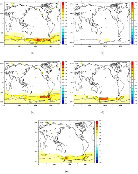
Figure 10 shows that the ocean surface temperature evolu-tion in the 30 kyr transient simulaevolu-tion is very close to equi-librium for all the parameter sets and resolutions we have tested. In addition, it shows that it is a robust result that ac-celerating the simulations up to a factor of 10 does not have a major effect on the global mean surface temperature. For the “Traceable” parameter set there is less difference between the accelerated and non-accelerated simulations than for the other three parameter sets. This is most likely related to the higher isopycnal and sea ice diffusivity in the “Traceable” pa-rameter set. Conversely, the “Low-diffusion” papa-rameter set results in a greater difference between the accelerated and non-accelerated simulations. This is unsurprising given the decrease in diapycnal diffusivity. These differences are high-lighted in Fig. 11, which shows the error in the×10 acceler-ated simulation, relative to the non-acceleracceler-ated simulation, at the LGM, for the four different parameter sets and the high resolution ocean. The “Traceable” parameter set, consistent with the idea that it has a shorter intrinsic timescale than the other sets, exhibits the smallest acceleration-error. How-ever, for all parameter sets and ocean resolutions we have investigated, the greatest acceleration-error is in the South-ern Ocean. Therefore, it appears to be a robust result that the Southern Ocean is the region most affected by the accelera-tion, and that the Northern Hemisphere, even with a factor of 10 acceleration, is relatively unaffected.

4 Discussion and conclusions

We have carried out equilibrium and transient simulations of the last 30 000 years with the GENIE-1 model. We find good agreement between our equilibrium simulations and previous work, although our model is not complex enough to simulate dynamical effects such as changes to the monsoons and there is a relatively large cold bias in our pre-industrial tropical surface temperatures. In our model, the time period from 30 kyrBP to pre-industrial is in very close equilibrium with the ice sheet, CO2, and orbital boundary conditions. This

implies that, negelecting fresh water forcing due to ice sheet fluctuations, the method of comparing equilibrium simula-tions with paleo data is not flawed in this respect.

Full complexity AOGCMs, such as the Met Office’s HadCM3, are currently too slow to carry out long transient

of speeding up a transient simulation is to accelerate the boundary conditions, and so compress the length of a sim-ulation. We find that the Southern Ocean and Antarctica are the regions most sensitive to this acceleration, where, for a×10 acceleration, errors in the annual mean surface tem-perature can be of the order 1–2◦C. However, the Northern Hemisphere is relatively insensitive to the acceleration. This implies that when comparing an accelerated AOGCM sim-ulation to paleodata, the Northern Hemisphere comparison, for example North Atlantic SSTs from dinoflagellates (e.g. de Vernal et al., 2005), is likely to be more robust than the Southern Hemisphere comparison, for example temperatures from Antarctic ice-cores (e.g. Petit et al., 1999). It also im-plies that transient simulations which aim to simulate pro-cesses in which the Southern Ocean plays a significant role, for example biogeochemical processes, should not be accel-erated. We have shown that these findings are independent of the particular parameter set we have used, and also hold when a higher vertical resolution is used in the ocean model. We believe that our results have significance beyond the GENIE-1 model. In an intercomparison study of several EMICs, Rahmstorf et al. (2005) found that all the 11 climate models tested, including GENIE-1 (named C-GOLDSTEIN in the Rahmstorf et al. paper), showed a qualitatively similar response to a transient fresh water forcing. This is different to the forcing applied in our study, but at least shows that GENIE-1 has associated typical timescales which are con-sistent with other EMICs. In a similar study, but one which included full-complexity GCMs in addition to EMICs, Stouf-fer et al. (2006) found that the oceanic response to a transient freshwater forcing was very similar in EMICs with a 3-D ocean and in full-complexity GCMs. In addition, we have shown that our LGM simulations are qualitatively similar to those produced using a model with a full complexity atmo-sphere. Coupled with the fact that our findings are indepen-dent of the resolution and parameter set used within GENIE-1, this leads us to believe that our conclusions about ac-celeration and transient/equilibrium simulations would hold in an identical experiment using a full-complexity GCM. However, those aspects of the simulations which depend on changes to cloud-cover, precipitation, or atmospheric circu-lation, such as the temperature anomaly at the mid-Holocene, would not be reproduced by a GCM.

Our experiments can help to guide the spin-up strategy of potential GCM transient simulations. Our results imply that a reasonable strategy would be to initially carry out an equilib-rium simulation of the start-point of the transient, and to use this as the initial condition for the transient. If this is done, then the results of the transient simulation can be considered spun-up after just a couple of decades.

(13)

Fig. 11. Annual mean surface temperature in the×10 accelerated 30 kyr simulation, relative to the non-accelerated simulation, at the LGM.

(a,b,c,d) are for the “Default”, “Traceable”, “Low-Diffusion”, and “Half-flux” parameter sets, respectively. (e) is for the “High-resolution”

(14)

tain initial conditions. By initialising the equilibrium simu-lations with an isothermal ocean, it is possible that we have preconditioned the ocean into a certain state. Possible fu-ture work could include initialising the transient simulations with “THC-off” ocean states, to see how this influences the results.

This work neglects the effects of some shorter-timescale transient events such as Heinrich events (Heinrich, 1988). These are events where there is thought to be an interaction between climate and ice sheets, which are not represented here. Work underway (Marsh et al., 2006) is investigating the effects of fresh-water pulses on the transient simulations presented in this paper.

Here we have only considered whether the ocean-atmosphere-sea ice-land surface system is close to equilib-rium with prescribed ice sheet and atmospheric CO2

bound-ary conditions, assuming fixed vegetation. The slow dynam-ics of ice sheets, the carbon cycle and other biogeochemi-cal cycles mean that these components of Earth system and hence the climate may be considerably out of equilibrium with orbital forcing. This remains to be investigated in future work, in particular with a version of the model being devel-oped, which includes dynamic vegetation, ice sheets (Payne, 1999), and biogeochemistry (Cameron et al., 2005).

Future work also includes a comparison of our transient simulations with the paleo record, and a study of the relative importance of the driving boundary conditions (ice sheet, or-bit, CO2) during the last 30 000 years.

Acknowledgements. This work was funded by the NERC

e-Science program through the Grid ENabled Integrated Earth system model (GENIE) project NER/T/S/2002/00217. We thank the NERC RAPID program NER/T/S/2002/00462 for providing the computer resources on which these simulations were carried out. We thank two anonymous reviewers for their useful and constructive comments. Many thanks to A. Yool who helped with the high-resolution simulations, and to M. Jones who improved the clarity of the language.

Edited by: N. Weber

References

Arnold, N. S., van Andel, T. H., and Values, V.: Extent and dynam-ics of the Scandinavian icesheet during Oxygen Isotope Stage 3 (60 000–30 000 yr BP), Quaternary Res., 57, 38–48, 2002. Berger, A.: Long-term variations of caloric insolation resulting

from the Earth’s orbital elements, Quaternary Res., 9, 139–167, 1978.

Cameron, D. R., Lenton, T. M., Ridgwell, A. J., Shepherd, J. G., Marsh, R., and Yool, A.: A factorial analysis of the marine car-bon cycle controls on atmospheric CO₂, Global Biogeochem. Cycles, 19, GB4027, doi:10.1029/2005GB002489, 2005.

parameter sensitivity in an efficient 3-D ocean-climate model, Clim. Dyn., 24, 415–433, 2005.

Fanning, A. G. and Weaver, A. J.: An atmospheric energy-moisture model: Climatology, interpentadal climate change and coupling to an ocean general circulation model, J. Geophys. Res., 101, 15 111–15 128, 1996.

Griffies, S. M.: The Gent-McWilliams skew flux, J. Phys. Oceanogr., 28, 831–841, 1998.

Haywood, A. M., and Valdes, P. J.: Modelling Pliocene warmth: contribution of atmosphere, oceans and cryosphere, Earth Planet. Sci. Lett., 218, 363–377, 2004.

Hargreaves, J. C., Annan, J. D., Edwards, N. R., and Marsh, R.: An efficient climate forecasting method using an intermediate complexity Earth System Model and the ensemble Kalman filter, Clim. Dyn., 23, 745–760, 2004.

Heinrich, H.: Origin and consequences of cyclic ice rafting in the northeast Atlantic Ocean during the past 130 000 years, Quater-nary Res., 29, 143–152, 1988.

Hewitt, C. D., Broccoli, A. J., Mitchell, J. F. B., and Stouffer, R. J.: A coupled model study of the last glacial maximum: Was part of the North Atlantic relatively warm?, Geophys. Res. Lett., 28, 1571–1574, 2001.

Hibler, W. D.: A dynamic thermodynamic sea ice model, J. Phys. Oceanogr., 9, 815–846, 1979.

Jackson, C. S. and Broccoli, A. J.: Orbital forcing of Arctic climate: mechanisms of climate response and implications for continental glaciation, Clim. Dyn., 21, 539–557, 2003.

Joos F., Gerber, S., Prentice, I. C., Otto-Bliesner B. L., and Valdes, P. J.: Transient simulations of Holocene atmospheric carbon dioxide and terrestrial carbon since the Last Glacial Maximum, Global Biogeochem. Cycles, 18, 2, GB2002, doi:10.1029/2003GB002156, 2004.

Jost, A., Lunt, D., Kageyama, M., Abe-Ouchi, A., Peyron, O., Valdes, P. J., and Ramstein, G.: High-resolution simulations of the last glacial maximum climate over Europe: a solution to discrepancies with continental paleoclimatic reconstructions?, Clim. Dyn., 24, 577–590, 2005.

Joussaume, S. and Taylor, K. E.: Status of the Paleoclimate Mod-elling Intercomparison Project (PMIP), in: Proceedings of the first international AMIP scientific conference, 425–430, 1995. Kaplan, J. O., Prentice, I. C., Knorr, W., and Valdes, P. J.:

Modeling the dynamics of terrestrial carbon storage since the Last Glacial Maximum, Geo. Res. Lett., 29(22), 2074, doi:10.1029/2002GL015230, 2002.

Lenton, T. M., Williamson, M. S., Edwards, N. R., Marsh, R., Price, A. R., Ridgwell, A. J., Shepherd, J. G., and the GENIE team: Millennial timescale carbon cycle and climate change in an effi-cient Earth system model, Clim. Dyn., 26, 687–711, 2006. Lorenz, S. J. and Lohmann, G.: Acceleration technique for

Mi-lankovitch type forcing in a coupled atmosphere-ocean circu-lation model: method and application for the Holocene, Clim. Dyn., 23, 727–743, 2004.

Marsh, R., Yool, A., Lenton, T. M., Gulamali, M. Y., Edwards, N. R., Shepherd, J. G., Krznaric, M., Newhouse, S., and Cox, S. J.: Bistability of the thermohaline circulation identified through comprehensive 2-parameter sweeps of an efficient cli-mate model, Clim. Dyn., 23, 761–777, 2004.

(15)

T. M., Williamson, M. S., and Yool, A.: Modelling ocean cir-culation, climate and oxygen isotopes in the ocean over the last 120 000 years, Clim. Past Discuss., 2, 657–709, 2006,

http://www.clim-past-discuss.net/2/657/2006/.

Monnin, E., Steig, E. J., Siegenthaler, U., Kawamura, K., Schwan-der, J., Stauffer, B., Stocker, T. F., Morse, D. L., Barnola, J. M., Bellier, B., Raynaud, D., and Fischer, H.: Evidence for sub-stantial accumulation rate variability in Antarctica during the Holocene, through synchronization of CO2 in the Taylor Dome, Dome C and DML ice cores, Earth Planet. Sci. Lett., 224, 45–54, 2004.

Payne, A. J.: A thermomechanical model of ice flow in West Antarctica, Clim. Dyn., 15, 115–125, 1999.

Peltier, W. R.: Ice-age paleotopology, Science, 265, 195–201, 1994. Petit, J. R., Jouzel, J., Raynaud, D., Barkov, N. I., Barnola, J. M., Basile, I., Bender, M., Chappellaz, J., Davis, J., Delaygue, G., Delmotte, M., Kotlyakov, V. M., Legrand, M., Lipenkov, V., Lo-rius, C., P´epin, L., Ritz, C., Saltzman, E., and Stievenard, M.: Climate and Atmospheric History of the Past 420 000 years from the Vostok Ice Core, Antarctica, Nature, 399, 429–436, 1999. Rahmstorf, S, Crucifix, M., Ganopolski, A., Goosse, H.,

Ka-menokovich, I., Knutti, R., Lohmann, G., Marsh, R., Mysak, L. A., Wang, Z., and Weaver, A. J.: Thermohaline circulation hysterisis: A model intercomparison, Geophys. Res. Lett., 32, L23605, doi:10.1029/2005GL023655, 2005.

Semtner, A. J.: A model for the thermodynamic growth of sea ice in numerical investigations of climate, J. Phys. Oceanogr., 6, 379– 389, 1976.

Stouffer, R. J., Yin, J., Gregory, J. M., Dixon, K. W., Spelman, M. J., Hurlin, W., Weaver, A.J., Eby, M., Flato, G. M., Hasumi, H., Hu, A., Junclaus, J. H., Kamenkovich, I. V., Levermann, A., Mon-toya, M., Murakami, S., Nawrath, S., Oka, A., Peltier, W. R., Robitaille, D. Y., Sokolov, A., Vettoretti, G., and Weber, S. L.: Investigating the causes of the response of the thermohaline cir-culation to past and future climate changes, J. Climate, 19, 1365– 1387, 2006.

Texier, D., de Noblet, N., and Braconnot, P.: Sensitivity of the African and Asian Monsoons to Mid-Holocene Insolation and Data-Inferred Surface Changes, J. Climate, 13, 164–181, 2000. de Vernal, A., Eynaud, F., Henry, M., Hillaire-Marcel, C.,

Lon-deix, L., Mangin, S., Matthiessen, J., Marret, F., Radi, T., Ro-chon, A. Solignac, S., and Turon, J.-L.: Reconstruction of sea-surface conditions at middle to high latitudes of the Northern Hemisphere during the Last Glacial Maximum (LGM) based on dinoflagellate cyst assemblages, Quaternary Sci. Rev., 24, 897– 925, 2005.

Weaver, A. J., Eby, M., Weibe, E. C., Bitz, C. M., Duffy, P. B., Ewen, T. L., Fanning, A. F., Holland, M. M., MacFadyen, A., Matthews, H. D., Meissner, K. J., Saenko, O., Schmittner, A., Wang, H., and Yoshimori, M.: The UVic Earth system climate model: Model description, climatology, and applications to past, present and future climates, Atmos.e-Ocean, 39, 361–428, 2001. Weber, S. L., Drijfhout, S. S., Abe-Ouchi, A., Crucifix, M., Eby, M., Ganopolski, A., Murakami, S., Otto-Bliesner, B., and Peltier, W. R.: The modern and glacial overturning circulation in the At-lantic ocean in PMIP coupled model simulations, Clim. Past Dis-cuss., 2, 923–949, 2006,

http://www.clim-past-discuss.net/2/923/2006/.

Williamson, M. S., Lenton, T. M., Shepherd, J. G., and Ed-wards, N. R.: An efficient numerical terrestrial scheme (ENTS) for Earth system modelling, Ecological Modell., 198, 362-374, 2006.