www.atmos-meas-tech.net/9/1181/2016/ doi:10.5194/amt-9-1181-2016
© Author(s) 2016. CC Attribution 3.0 License.
Lidar-Radiometer Inversion Code (LIRIC) for the retrieval of
vertical aerosol properties from combined lidar/radiometer data:
development and distribution in EARLINET
Anatoli Chaikovsky1, Oleg Dubovik2, Brent Holben3, Andrey Bril1, Philippe Goloub2, Didier Tanré2,
Gelsomina Pappalardo4, Ulla Wandinger5, Ludmila Chaikovskaya1, Sergey Denisov1, Jan Grudo1, Anton Lopatin1, Yana Karol1, Tatsiana Lapyonok2, Vassilis Amiridis6, Albert Ansmann5, Arnoud Apituley7,
Lucas Allados-Arboledas8, Ioannis Binietoglou9, Antonella Boselli10,4, Giuseppe D’Amico4, Volker Freudenthaler11, David Giles3, María José Granados-Muñoz8, Panayotis Kokkalis6,12, Doina Nicolae9, Sergey Oshchepkov1,
Alex Papayannis12, Maria Rita Perrone13, Alexander Pietruczuk14, Francesc Rocadenbosch15, Michaël Sicard15, Ilya Slutsker3, Camelia Talianu9, Ferdinando De Tomasi13, Alexandra Tsekeri6, Janet Wagner5, and Xuan Wang10 1Institute of Physics, NAS of Belarus, Minsk, 220072, Belarus
2LOA, Universite de Lille, Lille, 59650, France
3NASA Goddard Spaceflight Center, Greenbelt, MA 20771, USA
4Consiglio Nazionale delle Ricerche – Istituto di Metodologie per l’Analisi Ambientale (CNR-IMAA), Potenza, 85050, Italy 5Leibniz Institute for Tropospheric Research, Leipzig, 04318, Germany
6Institute for Astronomy, Astrophysics, Space Applications and Remote Sensing, National Observatory of Athens, Athens, 15236, Greece
7KNMI – Royal Netherlands Meteorological Institute, De Bilt, 3731, the Netherlands
8Andalusian Institute for Earth System Research (IISTA-CEAMA), University of Granada, Autonomous Government of Andalusia, Granada, 18071, Spain
9National Institute of R&D for Optoelectronics, Magurele, 77125, Romania
10Consorzio Nazionale Interuniversitario per le Scienze Fisiche della Materia, Naples, 80138, Italy 11Ludwig-Maximilians Universität, Meteorological Institute, München, 80539, Germany
12National Technical University of Athens, Department of Physics, Athens, 15780, Greece 13Consorzio Nazionale Interuniversitario per le Scienze Fisiche della Materia (CNISM) and Universita’ del Salento, Lecce, 73100, Italy
14Institute of Geophysics, Polish Academy of Sciences, Warsaw, 01-452, Poland
15Remote Sensing Laboratory (RSLAB), Department of Signal Theory and Communications, Universitat Politècnica de Catalunya (UPC)/Institute for Space Studies of Catalonia (IEEC), Barcelona, 08034, Spain
Correspondence to: Anatoli Chaikovsky ([email protected])
Received: 19 October 2015 – Published in Atmos. Meas. Tech. Discuss.: 7 December 2015 Revised: 17 February 2016 – Accepted: 29 February 2016 – Published: 21 March 2016
Abstract. This paper presents a detailed description of LIRIC (LIdar-Radiometer Inversion Code) algorithm for si-multaneous processing of coincident lidar and radiometric (sun photometric) observations for the retrieval of the aerosol concentration vertical profiles. As the lidar/radiometric in-put data we use measurements from European Aerosol Re-search Lidar Network (EARLINET) lidars and collocated
aerosol layer as a priori constraints. The use of polarized li-dar observations allows us to discriminate between spherical and non-spherical particles of the coarse aerosol mode.
The LIRIC software package was implemented and tested at a number of EARLINET stations. Intercomparison of the LIRIC-based aerosol retrievals was performed for the obser-vations by seven EARLINET lidars in Leipzig, Germany on 25 May 2009. We found close agreement between the aerosol parameters derived from different lidars that supports high robustness of the LIRIC algorithm. The sensitivity of the re-trieval results to the possible reduction of the available ob-servation data is also discussed.
1 Introduction
The aerosol impact on the radiation balance of the atmo-sphere is an important climate forcing factor. In addition, aerosol particles are among the unhealthiest air pollutants. This is made more severe by rapid propagation of pollutants in the atmosphere that expands local ecocatastrophes to a global scale. Therefore, the monitoring of the aerosol evo-lution and transport in the atmosphere is an obligatory pre-requisite for predicting climatic and ecological changes.
Sun-radiometer and lidar networks contribute to aerosol remote sensing. The global Aerosol Robotic Network (AERONET) of ground-based sun–sky-scanning radiome-ters (e.g. Holben et al., 1998) provides reliable data on columnar aerosol properties from more than 200 globally dis-tributed sites. The results of AERONET observations are the aerosol optical thickness (AOT) obtained from direct sun ob-servations and additional microphysical and optical proper-ties of aerosol particles (single scattering albedo, volume dis-tribution of aerosol particles, complex refractive index, frac-tion of spherical particles, etc.) derived by the inversion of direct and scattered radiation measurements (Dubovik and King, 2000; Dubovik et al., 2002, 2004). The regional ra-diometer network SKYNET was established in the south-eastern Asian regions (Takamura et al., 2004), and it employs its own equipment and processing procedure (Hashimoto et al., 2012).
The lidar measurements are used to provide information on the vertical variability of the aerosol characteristics. Cur-rently, lidar networks, such as the European Aerosol Re-search Lidar Network (EARLINET) (Bösenberg et al., 2000; Pappalardo et al., 2014), the micro-pulse lidars network (MPL-Net) (Welton et al., 2002), the Asian dust network (AD-Net) (Murayama et al., 2001), the lidar network in for-mer Soviet Union countries CIS-LiNet (Chaikovsky et al., 2005), the northeast American CREST Lidar Network (CLN) (Hoff et al., 2009), and the Latin America Lidar Network LA-LINET (Antuña et al., 2012), monitor aerosol vertical dis-tributions in the atmosphere over vast regions of the Earth. The Global Atmosphere Watch (GAW) Aerosol Lidar
Ob-servation Network (GALION), also known as the “network of networks” (e.g. Bösenberg and Hoff, 2007), was estab-lished under the aegis of GAW to coordinate lidar activity all over the world. The outcome of the lidar observations are presented in the lidar network databases as vertical profiles of aerosol backscatter and extinction coefficients.
Aerosol columnar properties from AERONET and afore-mentioned vertical profiles of aerosol parameters from lidar networks are complementary pieces of information charac-terizing aerosol properties. Nowadays, lidars and sun–sky-scanning radiometers are among the basic tools in compre-hensive experiments aimed at studying the transformation and transport of smoke (e.g. Lund Myhre et al., 2007; McK-endry et al., 2011; Colarco et al., 2004), dust (e.g. Ansmann et al., 2009; McKendry et al., 2007; Müller et al., 2003; Pa-payannis et al., 2008), and volcanic ash (e.g. Ansmann et al., 2010, 2011, 2012; Papayannis et al., 2012; Gasteiger et al., 2011). A number of SKYNET sites (Takamura et al., 2004) and most of the EARLINET stations are equipped with li-dar and radiometer instruments. Further enhancement of the aerosol characterization is expected from the synergy of co-located radiometer and lidar observations. Namely, the coor-dination of measurement procedures of the two systems and the derivation of aerosol parameters from combined mea-surements results in advanced characterization of the aerosol layer with a superior performance compared to the aerosol information that would have been obtained from independent processing of lidar and radiometer data.
The idea of combined lidar and radiometer sound-ing (LRS) for retrievsound-ing vertical distributions of aerosol char-acteristics was first proposed by Chaikovsky et al. (2002), and it gave rise to the development of the lidar–radiometer synergetic algorithms (e.g. Chaikovsky et al., 2004a, b). Later, in 2012 under the ACTRIS Research Infrastructure project within the European Union Seventh Framework Pro-gramme, the algorithm and software package, named LIRIC (LIdar-Radiometer Inversion Code), was developed for pro-cessing data of EARLINET measurements. LIRIC is based on processing co-located lidar and radiometer measurements by using a two-step sequential inversion. First, the radiome-ter data was processed according to the standard AERONET inversion algorithm. Then, first-step results are used as a pri-ori constrains on aerosol properties for lidar data processing. First application of LIRIC technique to the actual data processing was presented by Chaikovsky et al. (2004a). In that study, the technique was adapted to the EARLINET-AERONET stations in Minsk (Belarus) and Belsk (Poland) (e.g. Chaikovsky et al., 2004c, 2010a; Pietruczuk and Chaikovsky, 2007). Results of the LRS observations were of interest for the study of long-range aerosol transport in the eastern European region (Kabashnikov et al., 2010; Chaikovsky et al., 2010b; Papayannis et al., 2014).
into log-normal modes and selection of some of these modes for the characterization of aerosol layers using measured li-dar data (Cuesta et al., 2008).
The LRS technique for retrieving the aerosol concentra-tion profiles from single-wavelength lidar measurements at the MPLNET (Micro-Pulse Lidar Network) stations collo-cated with the sun–sky radiometer sites of AERONET was developed by Ganguly et al., 2009a. Then this method was applied to processing of the combined AERONET and space CALIOP lidar data (Ganguly et al., 2009b).
Besides, the single-wavelength POLIPHON technique was developed as an alternative (e.g. Tesche et al., 2009; Ansmann et al., 2012). This technique retrieves particle vol-ume concentration profiles of aerosol separately for fine and coarse fractions. The algorithm relies on the measured pro-files of the particle linear depolarization ratio and lidar ratio, and it does not require the assumption of a specific particle shape. Columnar concentrations of aerosol modes retrieved by AERONET are used in POLIPHON as additional input data. The algorithm POLIPHON is designed for the data pro-cessing in lidar sounding of the aerosol layers with coarse non-spherical particles (dust, volcano ash).
In recent years, the LRS technique has been implemented within the advanced research network ACTRIS in the frame of EU 7th Framework Programme project. To date, a number of joint EARLINET/AERONET stations have implemented regular atmospheric observations using LIRIC for process-ing combined sun-radiometer and lidar-measured data (e.g. Chaikovsky et al., 2012; Papayannis et al., 2014; Tsekeri et al., 2013). The aerosol model and mathematical basis of the LIRIC algorithm became the prerequisite for further develop-ment of algorithms for simultaneous inversion of combined lidar–radiometer measurements, e.g. GARRLIC (General-ized Aerosol Retrieval from Radiometer and Lidar Combined data) (Lopatin et al., 2013) and the results of ground/satellite closure experiments (Dubovik et al., 2014). Note that LIRIC technique should not be regarded only as a basis for new al-gorithms (e.g. POLIPHON or GARRLIC). LIRIC might be superior to them for many aerosol scenarios: it allows one, for example, to distinguish between fine and coarse spherical fractions (unlike POLIPHON) or distinguish between spher-ical and non-spherspher-ical coarse particles (unlike GARRLIC). At the same time, a comprehensive description of the LIRIC algorithm has not been yet documented in detail.
This paper describes the basic physical and mathematical aspects of LIRIC algorithm with all necessary equations, thus filling up this gap. The appendices contain the details of the inversion scheme and can be useful for advanced users to modify and improve this code.
2 The algorithm concept and structure
The aerosol retrievals from combined lidar and radiometer measurements belong to a class of “ill-posed” inverse prob-lems that, in particular, is characterized by non-unique and
highly unstable solutions arising even under small measure-ment or simulation errors. In practice, the solution of the “ill-posed” problems requires the introduction a priori informa-tion (e.g. Turchin et al., 1971; Tikhonov and Arsenin, 1977; Twomey, 1977; Tarantola, 1987; Rodgers, 2000). LIRIC al-gorithm was designed on the basis of multi-term LSM (least square method) (Dubovik, 2004). This method was imple-mented in AERONET data processing (Dubovik and King, 2000) and then it was refined in the retrieval algorithms for the data processing of the combined optical measurements (e.g. Dubovik, 2004; Dubovik et al., 2011, 2014; Lopatin et al., 2013).
The inversion algorithm LIRIC can be divided into three key procedures (e.g. Tarantola, 1987): (i) parameterization of the object under study (i.e. development of the aerosol layer model); (ii) forward modelling, i.e. derivation of the equa-tions that relate observed signals with specified parameters of the aerosol model; and (iii) inverse modelling or retrieval of the target parameters of the aerosol model that minimize discrepancies between the measured and the calculated input signals.
2.1 Combined lidar/radiometer experiment and aerosol model
The lidar/radiometer input data assumed to come from measurements of EARLINET lidars (e.g. Matthias et al., 2004; Freudenthaler et al., 2010) and spectral-scanning sun-radiometers of AERONET (Holben et al., 1998). The ma-jority of EARLINET lidar stations provides daytime mea-surements of elastic backscatter signals at three wavelengths (355, 532, and 1064 nm) and two cross/parallel-polarization components of the signal at a single wavelength. Additional information on aerosol parameters is expected to come from daytime Raman lidar measurements. (The current version of LIRIC algorithm is not designed for using Raman lidar data.) Radiometric data includes results of direct-sun and al-mucantar (scanning) measurements (Holben et al., 1998; Dubovik and King, 2000). Direct-sun measurements are carried out in 15 min intervals. Almost-clear-sky measure-ments are required to obtain almucantar data, and approx-imately two to six successful measurements are made dur-ing the daytime under favourable meteorological conditions at EARLINET/AERONET stations. Under these circum-stances, time synchronization of lidar and radiometric ob-servations usually means nearly simultaneous measurements within the same 1 h interval.
desirable to perform the lidar sounding from the lowest pos-sible altitude. Likewise, the contribution of the bottom layer (which is not observed by lidar) to the columnar optical pa-rameters must be small enough to be modelled by a homoge-neous layer with the same aerosol parameters as at the lowest level of lidar sounding. In practice, the lower sounding limit for most of the lidar measurements in EARLINET is about 200 m or more that can be too high especially for low bound-ary layers in winter seasons. It should be decreased in winter to compensate reduction of the boundary layer height. There-fore, lidar measurements in the lower layer have to be car-ried out by a second, complementary receiving system with smaller objective and larger field of view or by sounding the atmosphere along a slant trajectory.
The choice of the optical aerosol model is a key step of the retrieval algorithm. The optical model should be constructed following the principle of parsimony or “Occam’s razor”: the number of aerosol parameters has to be minimal but com-plete in order to provide unbiased retrieval from available measurements.
In this work, we use the AERONET model approach to characterize the aerosol layer of the atmosphere (Dubovik and King, 2000): aerosols are modelled by several modes with a certain aerosol particle size distribution, wherein each mode is a mixture of homogeneous spherical particles and randomly oriented spheroids (Dubovik et al., 2002, 2006). The distribution of the spheroid aspect ratio is fixed. The number of aerosol modes,K, depends on specification of the lidar data. If we use only total (scalar) backscatter lidar mea-surements, the aerosol model includes fine and coarse modes (K=2). There is boundary size between fine and coarse fractions in the algorithm, which is determined as the value in 0.194–0.576 µm range that corresponds to a minimum of the column particle volume size distribution, dV (r)/d lnr. If measurements of cross and parallel co-polarized compo-nents are available, spherical and non-spherical particles of the coarse mode are considered as two different fractions (K=3).
Thus, two sets of parameters characterize the aerosol layer. 1. The first is a number of columnar aerosol parameters retrieved from radiometer measurements (Dubovik and King, 2000; Dubovik et al., 2002, 2006). This set of pa-rameters is formed by the following: (1) the total content of each aerosol mode, (i.e. columnar volume concentra-tions),
ˆ
CkV =
rmax,k
Z
rmin,k dVk(r)
d lnr d lnr, (1)
where rmin, k and rmax, k is the minimum and the
maximum radius of the kth aerosol mode (k=
1, . . ., K) , respectively; (2) the particle volume
size distributiondVk(r)/d lnr for each aerosol mode;
(3) complex refractive indices at the wavelength λ,
m (λ)=n (λ)+iκ (λ); (4) the “sphericity”, ζsph (the
ratio of spherical particle’s volume to the total vol-ume); (5) aerosol optical thickness (AOT) of the kth aerosol mode,Eˆk λj; (6) the single scattering albedo
for thekth aerosol mode, $k(λ); (7) the elements of
the backscattering matrix,Px,xk (λ,180◦); and (8) coeffi-cients akand bk, which determine optical extinction and
backscatter characteristics of aerosol particles for thek -aerosol mode (see Sect. 3.1). Parameters (1)–(4) are the independent “state” variables, whilst parameters (5)–(8) are derived from the state variables. Parametersm(λ)
andζsphare assumed the same for particles of all sizes. Definitions and a detailed description of the columnar aerosol parameters are available at the AERONET in-formation system; cloud screening and quality control algorithms were described by Holben et al. (2006). 2. The second set of parameters is represented by the
height, h, distributions of particle volume concentra-tions (PVC) for each of aerosol mode,ck(h), which
de-fine the vertical variability of the aerosol features. A lack of lidar data to resolve height-variation of aerosol microstructure motivates the assumption of altitude-independent microphysical parameters of the aerosol modes. 2.2 Algorithm’s structure
Two options of the retrieval procedure for the processing LRS data have been developed:
1. First one deals with sequential inversion of lidar and ra-diometer data. It is carried out by preliminary calcula-tion of the column parameters defined in Sect. 2.1 from radiometric measurements by using the AERONET in-version algorithm (Dubovik and King, 2000), followed by subsequent inversion of the height distribution pa-rameters by using lidar data with columnar characteris-tics of aerosol layer passed as a priori data (Chaikovsky et al., 2012);
2. Second option suggests simultaneous inversion ap-proach for retrieving optimal parameters of the aerosol model by using a joint inversion procedure from com-bined lidar and radiometer data.
and calculated input signals are obtained from both retrieval procedures when processing experimental data (Lopatin et al., 2013).
Advantages of the “simultaneous inversion approach” are expected for more involved measurements, such as in the unified algorithm GRASP (Generalized Retrieval of Aerosol and Surface Properties), which aimed at characterizing atmo-spheric properties from remote ground and satellite observa-tions (Dubovik et al., 2014).
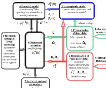
LIRIC algorithm described below was created on the base of the sequential inversion approach. Figure 1 shows the structure of the algorithm.
The algorithm is divided into several rather independent modules to provide flexibility of the software package. Mod-ule 1 (preprocessing of lidar data) creates a set of smoothed and normalized lidar signals, L∗, covariance matrix, L,
and setting parameters (type of lidar measurement, sound-ing wavelength, geographical coordinates of lidar station and date of measurement, etc.) for modelling aerosol and molec-ular layers. Module 2 (recalculation of radiometer data) es-timates columnar parameters of the aerosol model for lidar sounding wavelengths. Level 1.5 or Level 2.0 AERONET data are acceptable as input data in LIRIC. (These data are inputs to Module 2). Initial profiles of the aerosol-mode concentrations, c0k(h), as well as molecular (Rayleigh) ex-tinction, σr(λ, h), and molecular backscatter coefficients,
βr(λ, h), are generated by Module 3 (atmospheric model).
Module 4 (forward model) calculates arrays of lidar sig-nals, Lj
cmk−1(h), and columnar volume concentrations, ˆ
CkV ,m−1, given aerosol concentration profiles, cmk−1(h), in iterative inversion procedure, where “m” stands for them -th retrieval iteration and “j” is the number of the receiving channel. Inversion parameters, constraints on the smoothness characteristics, and error signals for the sensitivity test are passed to the algorithm by Module 5 (inversion settings & er-ror modelling). The sensitivity test (see Sect. 6) was de-signed to estimate the response of the retrieval results to measurement errors and/or uncertainties of input data. Mod-ule 6 (numerical inversion) is responsible for fitting aerosol-mode concentration profiles for the retrieved aerosol aerosol-model,
cmk−1(h), given measured data and a priori information. 3 Forward modelling of LRS experiment
Range-corrected normalized lidar signals and columnar-aerosol parameters retrieved from radiometer measurements are the input data to the LRS processing procedure (see Fig. 1). Below, we define a set of basic equations that are needed for the forward modelling of the measured quantities as well as to estimate the error-covariance matrix.
3.1 Basic lidar equations
The multichannel lidar carries out J “different” lidar mea-surements (j∈1, . . .J ) that yields a set of lidar signal
records,Pj∗,j ∈1, . . .J. The term “different” means that dif-ferent kinds of lidar measurements are performed, such as total intensity as well as cross- and parallel-polarized sig-nal components at different wavelengths. Here we consider that each “different” lidar measurement is provided by a spe-cificj-th channel. ParameterJ stands for the number of lidar channels irrespective of the actual implementation of the li-dar system.
Range-corrected normalized lidar signals are calculated at the preprocessing stage of the inversion procedure (Module 1 in Fig. 1):
L∗j(h)=
Sj∗ λj, h
ˆ
Sj∗(λ, href)
exp −2τr(λj, h, href), (2)
whereSj∗ λj, h=Pj∗(λj, h)h2;Sˆj∗ λj, hrefis the value of
Sj∗ λj, h
at the reference point,hrefis usually defined in the end of the sensing range,τr(λj, h, href)is the molecular opti-cal thickness related to the range of(h, href),λjis the
wave-length, andhis the height. The set of lidar signals,L∗j(h), constitutes the input lidar vector,L∗.
The lidar system provides measurements from the lowest to the highest altitude levels specified byhminandhmax, re-spectively. Currently, it is assumed that the radiometer is co-located at a height ofh0< hmin, so columnar aerosol opti-cal properties of the layerh0< h < hminare to be taken into consideration. If there is no information on the aerosol pa-rameters in the surface layer, this layer is assumed to be ho-mogeneous. Under this assumption, scattering parameters for the altitude rangeh0< h < hminof the lidar vectorL∗are set equal to the values athmin.
The relationship between the measured lidar signals
L∗(λ) and the aerosol mode concentration, ck(h), can be
written as follows:
L∗=L (λ, ck(h),ak,bk)+1L, (3)
where1Lis the vector of measurement uncertainties. Here,
an asterisk (*) denotes “measured” and no-asterisk denotes “model estimated”.
Since functionL (. . .)in Eq. (3) depends on the type of li-dar measurement, it is expedient to introduce special param-eter,pj∈1,2, . . ., U, that indicates the type of measurement
associated to thej-channel of the lidar, andUis a number of the types. In our case,pj∈1,2,3, indicates total intensity,
cross-polarized, and parallel-polarized measurements, corre-spondingly.
Figure 1. Flowchart of LIRIC algorithm. Details are in Sect. 2.2.
by the equation for the total backscatter signal,
Lj,1 λj, h=
βa,1(λj, h)+βr(λj, h)
Rj,1(λj, href)βr(λj, href)
exp
−2
h Z
href
σa(λj, h)dh
, (4)
where
Rj,1(λj, h)=
βa,1(λj, h)+βr(λj, h)
βr(λj, h)
; (5)
by the equation for the parallel-polarized signal component,
Lj,3 λj, h=
βa,3(λj, h)+1+1χβr(λj, h)
1
1+χβr(λj, href)Rj,3(λj, href)
exp
−2
h Z
href
σa(λj, h)dh
, (6)
where
Rj,3(λj, h)=
βa,3(λj, h)+1+1χβr(λj, h)
1
1+χβr(λj, h)
; (7)
and by the equation for the cross-polarized signal compo-nent,
Lj,2 λj, h
=
βa,2(λj, h)+µβa,3(λj, h)+χχ++µ1βr(λj, h)
χ+µ
χ+1βr(λj, h)Reff(λj, href)
exp
−2
h Z
href
σa(λj, h)dh
, (8)
where
Reff(λj, h)=
χ
(χ+µ)
βa,2(λj, h)+χχ+1β,r(λj, h)
χ
χ+1βr(λj, h)
+ µ
(χ+µ)
βa,3(λj, h)+1+1χβr(λj, h)
1
1+χβr(λj, h)
!
. (9)
In Eqs. (4)–(9), βa,1, βa,3, and βa,2 denote the aerosol backscatter coefficient and its parallel- and cross-polarized components, respectively; σa(λj, h) is the aerosol
extinc-tion coefficient; χ λj=ββr,2(λj)
r,3(λj) is the ratio of cross- and parallel-polarized components of the molecular backscatter coefficient.
in-clude the residual of cross-polarized component of the laser beam, non-ideal adjustment of the polarization planes be-tween transmitter/receiver channels and depolarization by optical elements. Equations (6) and (8) allow for these cross-talk effects in a similar manner to Chaikovskii (1990) and Biele et al. (2000). Thus, parameterµin Eqs. (8)–(9) repre-sents the leakage of the parallel component of the sounding beam into the cross-polarized lidar receiving channel. Param-eterµis an instrument characteristic that is assumed to be a known quantity; i.e. it is not updated by the retrieval proce-dure.
The aerosol extinction and backscatter coefficients in the Eqs. (3)–(9) are expressed as a function of the parameters of the following aerosol modes:
σa(λj, h)=
X
k
ck(h)ak(λj), (10)
βa,1(λj, h)=
X
k
ck(h)bk,1(λj), (11)
βa,2(λj, h)=
X
k
ck(h)bk,2(λj), (12)
and
βa,3(λj, h)=
X
k
ck(h)bk,3(λj). (13)
The coefficientsak(λj)andbk,x(λj), pointed out in Sect. 2.1,
are determined by columnar optical parameters of aerosol modes:
ak(λj)=
ˆ
Ek(λj)
ˆ
CkV , (14)
bk,1(λj)=
1
4π$k(λj)ak(λj)P k
1,1(λj,180◦), (15)
bk,3(λj)=
1
4π$k(λj)ak(λj)
P1k,1(λj,180◦)+P2k,2(λj,180◦)
2 , (16)
bk,2(λj)=
1
4π$k(λj)ak(λj)
P1k,1(λj,180◦)−P2k,2(λj,180◦)
2 , (17)
where Eˆk is aerosol optical thickness for the kth aerosol
mode, $k(λ) is the single scattering albedo for the kth
aerosol mode, and Px,xk (λ,180◦) are the elements of the backscattering matrix.
3.2 Forward model of radiometer data
In accordance with the multi-term LSM approach (Dubovik, 2004), the columnar concentrations of aerosol modes, CˆVk,
obtained from radiometer measurements are formally con-sidered in LIRIC as a result of additional independent mea-surements.
The equation for the vector,Cˆ∗V, which is defined as the “measured” columnar volume concentrations of the aerosol modes given vector of aerosol modes concentration,c(hi),
i∈1, . . .I, can be written in the following form:
ˆ
C∗V =Hc+1V, (18)
where H is convolution matrix for summing the height-resolved concentration over the column;1V is the vector of
ˆ
C∗V uncertainties.
Thek-th component of the vector Cˆ∗V is defined by the following equation:
Ck∗V(ck(hi))=
I X
i=1
ck(hi)1hi+1V ,k. (19)
The structure of the vectorsCˆ∗V,c, and matrix H is consid-ered in Appendix C.
4 Numerical inversion
Statistical regularization technique (e.g. Turchin et al., 1971; Tarantola, 1987; Rodgers, 2000) considers errors, 1L and 1V, in Eqs. (3) and (18) as random variables. Under the
ad-ditional assumption that errors have independent normal dis-tributions, the multidimensional conditional probability den-sity function (PDF) (or “likelihood function”) is defined by Chaikovsky et al. (2004a)
FL∗,Cˆ∗V
c
∼exp
−1
2
L∗−L(c)T −L1
L∗−L(c)+Cˆ∗V−HcT
−V1Cˆ∗V−Hc
. (20)
Here,FL∗,Cˆ∗V c
is the PDF of measurement vectors
L∗andCˆ∗V,L(c)is the vector function in Eq. (3), H is the
matrix in Eq. (18),cis the target retrieval vector of aerosol modes concentration, andLandV are the covariance
ma-trices of error vectors1Land1V, respectively.
An extensively used tool for the regularization of an “ill-posed” problem is the application of a priori constraint on the smoothness of retrieved characteristics. LIRIC restricts the norms of the second differences of functionsck(hi).
Fol-lowing the statistical regularization approach (Turchin et al., 1971) we included a priori probability function,
Fapr(c)∼exp
−1
2
cTSc
(21) into the retrieval procedure as the additional constraint. Here,
S=ST2Q
−1
the second-order differences, and Q2 is diagonal weighting matrix (Twomey, 1977; Dubovik et al., 2011).
The Bayes’ strategy (Turchin et al., 1971; Tarantola, 1987; Rodgers, 2000) for solving an “ill-posed” problem combined with multi-term LSM technique (Dubovik, 2004; Dubovik et al., 2011) defines the solution cˆ in accordance with the maximum a posteriori rule
ˆ
c=arg min c {9(c)},
where the objective or cost function,9(c), has the follow-ing multi-term representation (Dubovik, 2004; Dubovik et al., 2011)
9(c)= L∗−L(c)T−L1 L∗−L(c)
+Cˆ∗V −HcTV−1Cˆ∗V −Hc +cTST2Q−21S2c
. (22)
We assume that the errors1Lin Eq. (3) and1V in Eq. (18)
are uncorrelated. In this case, the non-zero diagonal elements of the covariance matricesLandV are the variances of
the elements of the vectors1Land1V, respectively.
Since the minimization procedure does not prescribe a residual value for9(c), it is convenient to reformulate weight matrices as follows (Dubovik, 2004):
˘ L=
1
ε2LL
; ˘V =
1
εV2V
; ˘S=
1
εS2S , (23)
whereε2L,ε2W, andε2Sare the first elements of the correspond-ing covariance matrices.
After substitution of the covariance matrices expressed through the weight matrices into Eq. (22) and multiplication it byε2L, the9(c)takes the form of the sum of three compo-nents:
˘
9(L∗,CˆV,c)= ˘9L(L∗,c)+γV9˘V(Cˆ∗V,c)+γS9˘S(c), (24)
where ˘
9L(L∗,c)= L∗−L(c)
T ˘
−L1 L∗−L(c), (25) is related to “lidar-measured” data, Eq. (3),
˘
9V(Cˆ∗V,c)=
ˆ
C∗V −HcT˘V−1Cˆ∗V −Hc, (26) is related to radiometer-measured data, Eq. (18),
˘
9S(c)=
cTSTQ˘−21Sc, (27)
is related to a priori information, Eq. (21),
γV =
εL2
ε2V ; γS=
ε2L
ε22. (28)
The coefficientsγV andγS are so-called Lagrange
multipli-ers that determine the weight of different contributors from each source of information (i.e. “measurements” and “a-priori” contribution) to the retrieval solution relative to the contribution of the first data source (sinceγL=1).
Equa-tions (22) and (24) are equivalent; however, Eq. (24) is more convenient for the analysis of the relative contribution from different data source.
If γV, γS→0, we return to a non-regularized solution
for vector c that is based solely on measured lidar data with the minimum discrepancy between measured and cal-culated input signals. This solution, however, could be non-physical, multivalued, and unstable. The possible solution space should be restricted by increasing the Lagrange mul-tipliers despite the fact that it results in increasing discrep-ancy between measured and model signal. The algorithms to determine the Lagrange multipliers by finding a reason-able compromise between the solution quality and the close-ness of the measured and model signals are described in Hansen (2001), Vogel (2002), and Doicu et al. (2010). The set of Lagrange multipliers is provided to LIRIC’s users along with software package. However, we do not consider this set as the ultimate one, and we allow it to be modified to meet user’s specifications.
The final step of the retrieval procedure is calculation of the concentration profilesck(hi)for each aerosol mode.
Ini-tial approximations c0k(hi) are set and stepwise improved
to provide the minimum of the objective function (Eq. 25). Increments are calculated by means of the Levenberg-Marquardt method (Levenberg, 1944; Levenberg-Marquardt, 1963).
The analytical expressions of the terms of Eq. (25), the co-variance matrices, and the details of the inversion procedure are described in Appendices A, B, and C.
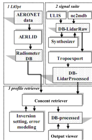
5 Program package for processing combined lidar and radiometer data
Figure 2 shows the structure of the software package that im-plements the LIRIC algorithm. A set of specific programs are joined in three sub-packages.
The sub-package LiOpt implements module (2) of the LIRIC algorithm (Fig. 1), which provides preprocessing of the AERONET retrieval products. Program AERLID re-calculates the columnar optical characteristics for the lidar sounding wavelengths, including the elements of the scatter-ing matrices for the spherical and non-spherical particles as well as for fine and coarse aerosol modes. Then, this code transfers data to the radiometer database.
The preprocessing of lidar data is carried out by the Sig-nalSuite sub-package. It contains several programs. Among them are the following:
Figure 2. Flowchart of the program package.
– nc2mdb – a program to convert EARLINET standard raw-lidar nc (network common data form) files into mdb (database file used by Microsoft Access) files to process by LIRIC;
– Synthesizer – a program to average the series of lidar signals, converts the profiles to the optimal altitude scale and, then, “glues” signals (i.e. synthesizes single signal) for the upper and lower troposphere, which were mea-sured with different receiving systems, as well as pro-vides the “dead-time” correction, i.e. the correction for the finite time resolution of the photo-counting system; – Tropoexport – a program to calculate a normalized smoothed lidar signal and its variance, and generates molecular and aerosol atmospheric models; this pro-gram aims at implementing modules 2 and 3 of the al-gorithm.
Finally, the main sub-package “ProfileRetriever” implements the LIRIC inversion procedure. The program “ConcentRe-triever” retrieves profiles cVk,m(h)of the aerosol mode con-centrations and writes data down to ACCESS database, DB-processed. The module “inversion setting & errors mod-elling” generates a set of noise-corrupted input data files by adding white noise and amplitude distortions to the initial lidar signals and perturbing aerosol model parameters re-trieved from radiometer measurements in order to provide the error sensitivity analysis. The user can upgrade default
instrumental noise parameters to meet real measurement con-ditions and technical features of the lidar system; the accu-racy of columnar aerosol parameters retrieved from the ra-diometer measurements (Dubovik and King, 2000; Dubovik et al., 2000) is also taken into account in setting parameters of the module. The program “OutputViewer” allows viewing the output data and their conversion from mdb-files into other formats.
6 Verification of operability and sensitivity tests The LRS technique uses the aerosol model that was ini-tially developed in AERONET to describe column-averaged aerosol properties and generalized it to the case of the height-resolved aerosol concentrations. This model assumes that aerosol consists of fine and coarse modes and that both are mixtures of spherical particles and randomly ori-ented homogeneous spheroids. The advanced T-matrix code (Mishchenko al., 2000, 2002) provides computation of scat-tering matrices of the aerosol particles. Thus, any optical characteristic of the aerosol layer can be calculated using data of the LRS experiment.
The applicability analysis of the AERONET spheroid model to aerosol particles is beyond the scope of this pa-per. We only note that this model was validated by the com-parison of calculated optical parameters and laboratory mea-surements of light scattering matrices for mineral dust par-ticles (Volten et al., 2001). Incorporation of the spheroid model into AERONET operational retrieval code has sig-nificantly improved AERONET products when evaluating parameters of coarse non-spherical particles (Cattrall et al., 2005; Dubovik et al., 2006). This model has also been incor-porated when processing data from ground-based polarimet-ric measurements (e.g. Li et al., 2009), lidar sounding data (e.g. Veselovskii et al., 2010; David et al., 2013; Müller et al., 2013), and satellite-base observations (e.g. Levy et al., 2007a, b; Dubovik et al., 2011; Schuster et al., 2012). 6.1 Verification of LIRIC program package: EARLI09
intercomparison experiment
EARLI09 intercomparison experiment was held in May 2009 at Leibniz Institute for Tropospheric Research in Leipzig, Germany (Wandinger et al., 2015). This campaign provided an excellent opportunity to validate the LRS technique for network measurements. The results of the LIRIC data pro-cessing for simultaneous measurements by seven lidars of different scientific teams on 25 May 2009 in Leipzig were compared.
Figure 3. EARLI09 intercomparison experiment: (a) NAAPS Total Optical Depth forecast, 25 May 2009 at 12:00 UTC; (b) 7-day back
trajectories ending over Leipzig, Germany at 12:00 UTC on 25 May 2009.
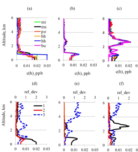
Figure 4. Particle volume concentrations (PVC) profiles,ck(h), and estimated deviations retrieved from data of EARLI09 intercompari-son campaign, 10:20–11:40 UTC, 25 May 2009, Leipzig, Germany, measured in Leipzig by six EARLINET lidars: mi – Minsk, ms – München, po – Potenza, bh – Bilthoven, hh – Hamburg, bu – Bucharest; (a, d) – fine, (b, e) – coarse spherical; (c, f) – coarse non-spherical; 1 – average PVC profile, 2 – rms-deviation (rms_dev), 3 – relative deviation (rel_dev). Measured data from four lidar channels (355, 532-parallel, 532-cross, 1064 nm) and three-mode aerosol model were used.
Figures 4 and 5 show PVC profiles,ck(h), retrieved from
lidar data of the different EARLINET teams combined with
(a) (b)
0 2 4 6
0 0.01 0.02 0.03
A
lt
it
u
d
e,
k
m
PVC, ppb mi ms po bh hh bu le
(c) (d)
0 1 2 3
0 2 4 6
0 0.01 0.02 0.03 rel_dev
A
lt
it
u
d
e,
k
m
PVC, r.m.s.dev; ppb 1 2 3
0 2 4 6
0 0.01 0.02 0.03 PVC, ppb
0 1 2 3
0 2 4 6
0 0.01 0.02 0.03
rel_dev
PVC, r.m.s.dev; ppb
Figure 5. Identical to Fig. 4 except for data from three lidar
channels (355, 532 – intensity/parallel polarized component, and 1064 nm) and two mode aerosol model were used. Label “le” stands for lidar “PollyXT” of TROPOS, Leipzig: (a, c) – fine, (b, d) – coarse spherical aerosol mode.
It is evident from Figs. 4a–c and 5a–b thatck(h)profiles
have similar structure over the troposphere except for the lower layer. The relative deviations increase mainly when values of the aerosol concentration become negligible. The discrepancies are also possible in the near-surface atmo-spheric layer due to overlap effect (e.g. for the Hamburg lidar system, Fig. 4a).
We explain the discrepancy betweenck(h)profiles in the
near-surface atmosphere by the uncertainty in geometrical overlap factors and the differences in lower-boundary heights of the considered lidar systems. Also some differences in the retrieved concentration profilesck(h)are due to
measure-ment errors and uncertainties in aerosol modelling.
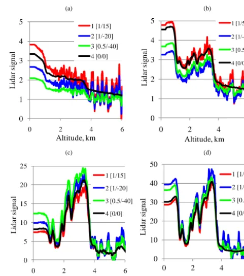
The potential errors in the PVC profiles for the specific combined lidar/radiometer experiment were estimated by using the Errors modelling module of the LIRIC package (Fig. 2). Figures 6 and 7 illustrate the sensitivity of the re-trieved aerosol concentration profiles to the errors of the lidar measurements. The original lidar signals were taken as they measured by München lidar (curves 4 in Fig. 6) and have been perturbed by adding white noise with different root-mean-square deviations (rms-deviations),αj, and have been
distorted by multiplying them by the coefficient,
kj(hi)=1+
1j
100
href−hi
href
, (29)
where percentage parameter 1j determines the amount of
non-linearity.
In response, the program module generated 12 disturbed lidar signal sets that allowed us to estimate the impact of measurement errors. As an illustration, Figs. 6 and 7 simu-late higher errors than typical sets in most EARLINET lidars. Four realizations of the disturbed signals are shown in Fig. 6. Coefficientkj(hi)increases/decreases from referent to start
point that results in divergence of the lidar signals in Fig. 6. PVC profiles,ck(h), corresponding to the lidar signals in
Fig. 6 and their rms-deviations calculated for full ensembles of input data are shown in Fig. 7. Changes in the PVC pro-files of the dominant coarse non-spherical mode are shown by the Fig. 7 to be minor (Fig. 7c). Although profilesck(h)
of fine and coarse spherical particles (Fig. 7a and b) are not very stable, they qualitatively retain similarity with the initial distributions.
Figure 8 illustrates the effect of uncertainties in columnar aerosol parameters retrieved from radiometer data. Variations of the columnar aerosol characteristics lead to changes in co-efficientsa andbof lidar-related Eqs. (14)–(17) (Sect. 3.1). Statistical characteristics of aerosol concentration profiles re-trieved with relative deviation of the parameterϑk,pj (effec-tive lidar ratio of the aerosol fraction, see Appendix B) in the range±20% (the full range) are presented in Fig. 8. Relative deviation of aerosol concentration profile becomes signifi-cant only for small values of the concentration.
(a) (b)
0 1 2 3 4 5
0 2 4 6
L
id
a
r
si
g
n
a
l
Altitude, km
1 [1/15] 2 [1/-20] 3 [0.5/-40] 4 [0/0]
(c) (d)
0 5 10 15 20 25
0 2 4 6
L
id
a
r
si
g
n
a
l
Altitude, km
1 [1/15]
2 [1/-20]
3 [0.5/-40]
4 [0/0]
0 1 2 3 4 5
0 2 4 6
L
id
a
r
si
g
n
a
l
Altitude, km
1 [1/5] 2 [1/-30] 3 [0.5/-20] 4 [0/0]
0 10 20 30 40 50
0 2 4 6
L
id
ar
si
g
n
al
Altitude, km
1 [1/-5]
2 [1/30]
3 [0.5/20]
4 [0/0]
Figure 6. Range-corrected normalized lidar signals,L∗, corrupted with noise and amplitude distortions. Original data are provided by the München lidar team in the frame of EARLI09 intercompari-son campaign, 14:30–15:30 UTC, 25 May 2009, Leipzig, Germany:
(a) – 355 nm, (b) 1064 nm, (c) – 532 nm, parallel polarized, (d) –
532 nm, cross polarized; 4 – original signal, 1–3 – corrupted
sig-nals. In square brackets distortion parametersαj/1jare given.
(a) (b) (c)
Figure 7. PVC profiles,ck(h), and their rms-deviations retrieved in response to disturbed data from of the München lidar, EARLI09 in-tercomparison campaign, 14:30–15:30 UTC, 25 May 2009, Leipzig, Germany: (a) – fine, (b) – coarse spherical, (c) – coarse non-spherical modes; 4 – for the original signal, 1–3 – for disturbed signals; 5 – rms-deviation.
6.2 Dependence of retrieved aerosol concentration profiles on the content of the input data set
(a) (b) (c)
0 1 2
0 2 4 6
0 0.005
rel_dev
A
lt
it
u
d
e,
k
m
c(h), rms_dev, ppb
1 2 3
0 1 2
0 2 4 6
0 0.005
rel_dev
c(h), rms_dev, ppb
0 1 2
0 2 4 6
0 0.015 0.03 rel_dev
c(h), rms_dev, ppb
Figure 8. Variations of PVC profiles, ck(h), retrieved with 20 % uncertainties in the aerosol lidar ratios; data of München lidar, EARLI09 intercomparison campaign, 14:30–15:30 UTC, 25 May 2009, Leipzig, Germany are used; (a) fine, (b) coarse spheri-cal, (c) coarse non-spherical modes; 1 – average value, 2 – rms-deviation, 3 – relative deviation.
measured lidar signals, column-aerosol parameters from ra-diometer measurements, and a priori smoothness constraints. Two- or three-mode aerosol models are used according to the type of the measured lidar signals. Formally, we deal with redundant input information and, hence, for the accepted aerosol model, the number of input data set can be decreased. Consequently, the significance of the different information components in retrieval procedure is of interest as well as variations of the retrieved profiles, ck(h), in the absence of
some input data
As pointed out in Sect. 4, the objective functions of LIRIC regularization algorithm (Eq. 22), consists of a set of terms that implement contribution of different types of input data into the retrieval process. Setting the variance of the specific kind of measurement to a large value implies neglecting the correspondent term in the objective function (Eq. 22) and the elimination of this part of the input data in estimation of the final aerosol parameters. Program package implements this option and makes allowing one to analyze the contribution of different measured data in the processing procedure of a specific experiment.
Below we shortly examine sensitivity of the retrieved pro-files,ck(h), to the input data selection for the case of
com-bined lidar/radiometer sounding of the atmospheric aerosol during the last period of Eyjafjallajökull volcano ash trans-port to the European area in Lille, France, on the 19 May 2010. Air mass back trajectories (Fig. 9) forecasted the pos-sibility of appearance of volcanic ash in the layer between 1300 and 2500 m. The structure of the retrieved profiles,
ck(h), shown in Fig. 10a agrees well with the forecast.
Devi-ations (by “deviDevi-ations” hereinafter we mean “standard devi-ation”) δ (ck(hi))associated to the profilesck(h)have been
calculated by an “error modelling” procedure similar to the one described in Sect. 6.1.
Figure 9. Air-mass back trajectories for Lille at 08:00 UTC, 19 May
2010, (NOAA HYSPLIT model).
(a) (b)
0 2 4 6 8
0 0.01 0.02
A
lt
it
u
d
e,
k
m
c(h), ppb fine coarse/sph coarse/nsph rms_dev(fine) rms_dev(coarse/sph) rms_dev(coarse/nsph)
0 2 4 6 8
0 0.05 0.1 0.15
Par. Dep. Ratio D(1) D(2) rms_dev(1) rms_dev(2)
Figure 10. (a), PVC profiles,ck(h), of the fine, course-spherical (coarse/sph) and coarse-nonspherical (coarse/nsph) aerosol modes, and their rms-deviations (rms_dev(fine), rms_dev(coarse/sph), and rms_dev(coarse/nsph)); (b), particle depolarization ratio, D(1) and (2), and their rms-deviations, rms_dev(1) and rms_dev(2). Profiles were retrieved from the data measured in Lille, 19 May 2010, 09:17–09:58 UTC. Profiles D(1) and rms_dev(1) are the results of the direct calculation of depolarization ratio and their rms-deviations from lidar measurements, as well as D(2) and rms_ev(2)
were calculated from retrieved aerosol mode concentrations,ck(h).
A mixture of spherical and non-spherical particles consti-tutes the aerosol layer at the height of about 2000 m. The profile of particle depolarization ratio at 532 nm and its de-viation have been calculated from the retrieved aerosol mode
(a) (b) (c)
0 2 4 6 8
0 0.01 0.02 0.03
A
lt
it
u
d
e,
k
m
c(h), ppb 355 532 1064 532-cross Cv Original
0 2 4 6 8
0 0.01 0.02 0.03 c(h), ppb
0 2 4 6 8
0 0.01 0.02 0.03
Тысяч
и
c(h), ppb
Figure 11. Variation of aerosol concentration profiles, ck(h), for fine (a), coarse spherical (b) and coarse non-spherical (c) aerosol modes in response to elimination of different parts of input informa-tion. Tag “Original” denotes complete set of input data; tag “355” (or 532, 1064, 532-cross) denotes that lidar signal at 355 nm (or 532,
1064, 532-cross) wavelength is excluded; tag “CV“ denotes that
columnar volume concentrations of aerosol modes are excluded. Lille, 08:00 UTC, 19 May 2010.
concentrations, ck(h). The profiles are shown in Fig. 10b,
curves D(2) and rms_dev(2). The results of the direct calcu-lation of depolarization ratio and their deviations from lidar measurements are presented by curves D(1) and rms_dev(1). It should be noted that the lidar measurements included ad-ditional calibration measurement that was not used by the retrieval procedure. Profiles D(1) and D(2) show rather close agreement in magnitude and vertical structure that could con-firm the efficiency of the aerosol modelling used in this study. The curves in Fig. 11 show the deviations in the retrieved concentration profiles,ck(h), after elimination one of the
li-dar signals or columnar volume concentrations of aerosol modes, CV, from the input data set. As can be seen from Fig. 11, the concentration profile of the fine-particle mode undergoes minor changes upon elimination of a single li-dar signal or the elimination of columnar volume concentra-tions. This could imply that our experiment initially included redundant input information, with respect to the fine-mode concentration. On the other hand, concentrations of coarse modes are sensitive to input information. Thus, lidar data at 1064 nm wavelength plays a crucial role in the retrieval of the coarse spherical mode. In the same manner, lidar depo-larization measurement is the key factor in the retrieval of the coarse spheroid particle mode. Evaluations of columnar vol-ume concentrations from radiometer measurement are nec-essary for all cases.
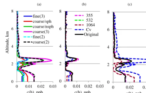
Figure 12a shows concentration profiles, ck(h), which
were retrieved for two- and three-mode aerosol models and characterized the aerosol layer in the same LRS experiment. The fine-mode concentration profiles for two aerosol mod-els are practically coincident. Profilesck(h)of coarse modes
(a) (b) (c)
0 2 4 6 8
0 0.01 0.02 0.03
A
lt
it
u
d
e,
k
m
c(h), ppb fine(3) coarse/sph coarse/nsph coarse(3) fine(2) coarse(2)
0 2 4 6 8
0 0.01 0.02 0.03 c(h), ppb
355 532 1064 Cv Original
0 2 4 6 8
0 0.02 0.04
c(h), ppb
Figure 12. Comparison of PVC profiles,ck(h), for the two- and three-mode aerosol models (a), and variations of concentration
pro-files,ck(h), for fine (b) and coarse (c) aerosol modes of the
two-mode aerosol two-model in response to elimination of different parts of input information. In Fig. 12a tags “fine(2)” and “coarse(2)” denote fine and coarse modes of two-mode aerosol model. Tags “fine(2)”, “coarse/sph”, “coarse/nsph” and “coarse(3)” denote fine, coarse spherical, course non-spherical and total course mode of three-mode aerosol model, correspondingly. In Fig. 12b and c tag “Original” means complete set of input data; tag “355” (or 532, 1064) denotes that the lidar signal at 355 nm (or 532, 1064)
wave-length is excluded; tag “CV“ denotes that columnar volume
concen-trations of aerosol modes are excluded. Lille, 08:00 UTC, 19 May 2010.
for two-mode aerosol model, coarse (2), and the sum of two coarse components for three-mode aerosol model, coarse (3), are similar in shape but quantitatively are a bit different. The column concentrations of the course (2) and (3) modes are equal.
The curves in Figs. 12b and c show the deviations of the concentration profiles,ck(h), for the two-mode aerosol
model after reduction of the input data set. Deviations of
ck(h)profiles are rather similar to those for the three-mode
aerosol model in Fig. 11. Deviations of fine-mode concen-tration profile are small, even if any single sub-set of input data is eliminated. Coarse-mode concentration profiles pre-serve original forms when one of the lidar signals at the 355 or 532 nm wavelength is excluded from the processing pro-cedure.
Generally, for measurement conditions that character-ize the experiment under discussion, two-wavelength lidar sounding (at 355 and 1064 or at 532 and 1064 nm) combined with radiometer measurement provides retrieving concentra-tion profiles of fine and coarse aerosol modes for two-mode aerosol model.
7 Discussion and conclusions
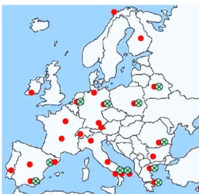
Figure 13. Map of the EARLINET stations (red dots). Green dots
indicate the stations where LIRIC program package has been im-plemented.
New scientific teams beyond EARLINET join the LIRIC user group. The detailed description of LIRIC algorithm and software in this paper should contribute to the effective im-plementation of the LRS technique by advanced users.
Retrieval of the aerosol parameters from the LRS mea-surements is an “ill-posed” inverse problem, and its solution should be tested on stability to the measurement errors and variations of the regularization parameters, which are set by the module “Inversion setting and errors moduling” of the software package (Fig. 2). Results of the EARLI09 intercom-parison experiment presented in Sect. 6.1 demonstrate rather small scatter in ck(h) profiles that were retrieved from the
data of different lidar systems with significantly corrupted in-put lidar signals and big uncertainties of the aerosol lidar ra-tio. This scatter is characterized by standard deviations of 5– 20 % of the maximum aerosol layer concentration. Increase inck(h)deviation in the bottom layer results from
uncertain-ties of the overlap function of the lidar systems.
The uncertainties in the retrieved aerosol parameters for different aerosol types, aerosol loads, overlap characteristics of the lidar systems and regularization parameters that are defined by the LIRIC operator were evaluated by Granados-Muñoz et al. (2014). The analysis covered combined lidar and radiometer measurements that were carried out during dust, smoke, and anthropogenic pollution events. This analy-sis mostly supports our conclusions on the stability of LIRIC solutions that retrieve basic aerosol features even under sig-nificant measurement errors. In particular, variations of the regularization parameters within one order interval from the original set lead to minor deviations of the retrieved ck(h)
profiles. Usually, it is unnecessary to change recommended utility regularization parameters while homogeneous input data sets are processed. The requirements for pre-processing
lidar signals along with the set of recommended regulariza-tion parameters are provided in the LIRIC user guide. How-ever, the utility parameters for error modelling menu should be defined by the LIRIC user with regard to the specific lidar system.
The requirement of having possibly minimal “full over-lap” height of lidar sensing is an important technical prob-lem for LRS measurements, because the near-surface aerosol layer contributes strongly to the radiometric data. In the ab-sence of lidar data, the surface aerosol layer is assumed to be homogeneous in the LIRIC aerosol modelling. Obviously, aerosol parameters can vary within the near-surface layer re-sulting in significant uncertainties in the LIRIC product, es-pecially when the lidar “dead zone” becomes comparable to the boundary-layer thickness. The effective solution of this problem is the set-up of a double lidar receiving block with special near-range channels for the detection of near-ground aerosol.
The analysis of the aerosol parameters that are retrieved from the incomplete sets of lidar data in Sect. 6.2 sup-ports the possibility to use LIRIC for processing data of wavelength lidar systems. Aerosol sounding by two-wavelength lidars, usually at 532 and 1064 nm two-wavelengths, is a widespread practice in atmospheric investigations. Sim-ulation results in Sect. 6.2 show the possibility to retrieve
ck(h) for two-mode aerosol model. The uncertainties of
such evaluatedck(h) are expected to surpass ones of
three-wavelength lidar sounding.
LIRIC implementation for the special lidar data set (532-cross, 532-parallel and 1064 nm) for retrieving parameters of the three-mode aerosol model is of interest for the satellite lidar CALIOP that provides similar lidar data (Winker et al, 2006).
Since the beginning of LIRIC dissemination in EAR-LINET community, experimental works on the validation of the LIRIC product for different aerosol types have being car-ried out. Comparisons of aerosol backscatter coefficients and depolarization ratios directly derived from lidar data against similar characteristics calculated from the aerosol optical and microphysical parameters retrieved by LIRIC (e.g. Tsekeri et al., 2012, 2013; Wagner et al., 2013; Kokkalis et al., 2013; Granados-Muñoz et al., 2014) as well as LIRIC against mod-elled or airborne in situ measured profiles of aerosol mode concentrations (e.g. Kokkalis et al., 2012, 2013; Nemuc et al., 2013) have shown reasonable agreement.
depolarization of backscatter signal to distinguish between spherical and non-spherical particles.
The number of aerosol studies using LIRIC algorithm increases. They focus on the investigation of the dynam-ics of aerosol microstructure during transport of air masses polluted by dust (e.g. Chaikovsky et al., 2010b; Tsekeri et al., 2013; Binietoglou et al., 2015; Granados-Muñoz et al., 2015a), fire smoke (e.g. Chaikovsky et al., 2010b; Granados-Muñoz et al., 2015b), volcano ash (Kokkalis et al., 2013) and anthropogenic pollution (Granados-Muñoz et al., 2014). LIRIC has become a tool for validation of the modelling
of aerosol transport in atmosphere (Binietoglou et al., 2015; Granados-Muñoz et al., 2015b). EARLINET teams form the data-base of the results of combined lidar and radiometer sounding.
Appendix A: General equation for received lidar signal Using general formula for received lidar signal instead of Eqs. (4), (6), and (8) allows us to derive compact and explicit expression for the covariance matrices,L, and regularizing
term,9˘L(L∗,c)(Sect. 4).
We will use the utility function
δpjj,u=
1...if . . ...pj =u
0...f . . .pj6=u ,
(A1) along with the following definitions of combinations of aerosol and molecular optical parameters in Eqs. (4)–(9):
βaef(λj, pj, h)= βa,pj(λj, h)
+δjp
j,2µβa,3(λj, h)
= X
k
ck(h)bk,pj(λj)
+δpj
j,2µ
X
k
ck(h)bk,pj(λj)
!
(A2)
βref(λj, pj, h)=
δjp
j,2(pj)
µ−1
χ+1
+ 1
1+δpj
j,3χ
βr(λj, h) (A3)
βef(λj, pj, h)=βaef(λj, pj, h)
+βref(λj, pj, h) (A4)
ˆ
Rjef(λj, pj, h)=
βaef(λj, pj, h)+βref(λj, pj, h)
βef
r (λj, pj, h)
(A5)
τa(λj, h, href)=
href Z
h
σa(λj, h)dh. (A6)
This permits Eqs. (4), (5) and (8) to be written in general form:
Lj pj, λj, h=
βef λj, pj, h
exp 2τa(λj, h, href)
βef
r (λj, pj, href)Rˆjef(λj, pj, href)
. (A7)
Therefore, the related to the lidar objective function, ˘
9L(L∗,c), (Eq. 25), is given by the equation:
˘
9L(L∗,c)=
X
j X
i
1hi
˘
Lj(i, i)
L∗j,i−
P
k
ck(hi)bk,p
j(λj)+δ
j p,2µ
P
k
ck(hi)bk,p
j(λj)
!
βref(λj, pj, href)Rˆef
j(λj, pj, href)
×exp 2P k
P
i
ck(hi)ak(λj)1hi !
2
i∈1, . . .I.
(A8)
Equation (26), 9˘V(Cˆ∗V,c), which brings radiometer data
into the processing procedure can be expressed as follows: ˘
9V(Cˆ∗V,c)=
X
k
1 ˘
V(k, k)
ˆ
C∗V−X
i
ck(hi)|1hi| !2
. (A9)
Calculation of the “smoothness” part of the objective func-tion is described in details in Dubovik, 2004; and Dubovik et al., 2011.
Appendix B: Evaluation of covariance matrixL The covariance matrixes, L, V, and 2, defined in
Sect. 4 characterize uncertainties of the complex input vec-tor,L∗,Cˆ∗V,0ˆ, where0 is “zero” vector that is defined toˆ formalize a priori smoothness restrictions on concentration profiles (e.g. Dubovik, 2004). These matrices determine the “weights” of different parts of input information through the minimization procedure of the objective function (Eq. 22).
In our case the measure of the smoothness for concentra-tion profiles,ck(hi), should be chosen as a priori evaluated
parameters. Aerosol columnar volume concentrations,Cˆ∗V, and variances, V(k, k), are the parts of input radiometer
data. Thus, only evaluation of covariance matrix,L, is to
be done.
The assumption of independent normal distribution for variations of “lidar” vector, L∗, at different heights im-plies the diagonal covariance matrix. The non-zero diag-onal elements, Lj(hi, hi), of the covariance matrix are the variances of differences between the components,L∗j,i, of the lidar vector and the appropriate modelled function,
Lj ck, pj, λj, hi
Given Eqs. (2), (3) and (A1)–(A-8), the elements of vector,
1Lj, are defined by the following:
1Lj(hi)=L
∗
j,i−Lj pj, λj, hi
= S
∗ λ
j, hi
ˆ
S∗ λ
j, href
exp(−2τr(λj, hi, href))
−β ef λ
j, pj, hiexp 2τa(λj, hi, href)
βef
r (λj, pj, href)Rˆefj(λj, pj, href)
. (B1)
Using the finite differences technique (e.g. Russell et al., 1979) one can expand1Lj(hi)in Taylor series, and then ne-glect all the terms of the second or higher order. As a re-sult, variationδ(1Lj(hi))can be expressed as a function of variations related with the input parameters,δ S∗ λj, hi, δ(βef(λj, pj, hi)),δ(τa(λj, hi, href), andδ(τr(λj, hi, href)):
δ(1Lj(hi))= −2L
∗
j,iδ(τr(λj, hi, href)) +L∗j,iδ S
∗ λ
j, hi
S∗ λ
j, hi
+β ef λ
j, pj, hiexp 2τa(λj, hi, href)
βef
r (λj, pj, href)Rˆefj(λj, pj, href)
δ βef λj, pj, hi
βef λ
j, pj, hi
−2β ef λ
j, pj, hiexp 2τa(λj, hi, href)
βef
r (λj, pj, href)Rˆjef(λj, pj, href)
δ(τa(λj, hi, href)
≈L∗j,i
δ S∗j(h i)
S∗j(h
i)
−δ β ef(λ
j, pj, hi)
βef(λ
j, pj, hi)
−2δ τr(λj, hi, href) −2δ τa(λj, hi, href)
. (B2)
Under the assumption of independent variations of differ-ent parameters, the varianceL(hi, hn)is expressed as
fol-lows
L(hi, hi)=
δ(1Lj(hi))δ(1Lj(hi))
=L∗j,n2 δ2
Pj,i∗
Pj,i∗
2 +
δ2 βef(λj, pj, hi)
βef(λj, pj, hi)
2
+4δ2 τr(λj, hi, href) +4δ2 τa(λj, hi, href)
, (B3)
whereh. . .idenotes ensemble averaging over measurement realizations, andPj,i∗ =Pj∗(hi).
The terms in the large round parentheses in Eq. (B3) deter-mine contributions of measurement errors and uncertainties
of a priori defined optical characteristics. We aim at approx-imate estimation ofLj(hi, hi)at the preprocessing stage without involving of retrieved parameters. This feedback-free approach greatly simplifies the structure of the inversion algorithm.
Uncertainties of the optical parameters The term δ2 βef
/ βef2
in Eq. (B3) is the relative vari-ance of the total backscatter coefficient. It can be transformed into the sum of relative variances of aerosol and molecular backscatter coefficients:
δ2 βef(λj, pj, hi)
βef(λ
j, pj, hi)
2 =
δ2 βref(λj, pj, hi)
βef
r (λj, pj, hi)
2 1
ˆ
Refj(λj, pj, hi) 2
+δ 2 βef
a(λj, pj, hi)
βef
a(λj, pj, hi) 2
ˆ
Refj(λj, pj, hi)−1 2
ˆ
Refj(λj, pj, hi)
2 . (B4)
The International Standard Atmosphere ISO 2533 and sea-sonal latitudinal changed model CIRA (Committee on Space Research (COSPAR), 2006; Fleming et al., 1988), as well as measurements by radiosondes are applied in LIRIC for the calculation of molecular optical parameters. The relative variance of calculated molecular backscatter coefficient
α12=δ
2 βef
r (λj, pj, hi)
βef
r (λj, pj, hi)2
(B5)
is assumed to be a constant and its value can be reduced to
α1=0.01 (e.g. Russell et al., 1979) if data of coordinated radiosonde measurements are available.
The aerosol backscatter coefficients, βaef(λj, pj, hi),
are estimated by using Eqs. (10)–(17). Uncertainties of
βaef(λj, pj, hi)basically follow from estimation errors of the
coefficientb(ν, j, pj)in Eqs. (15)–(17) that can be written
by the equation:
b(j, pj, k)=
1
ϑk,pj
Ek∗ λj
ˆ
CkV , (B6)
where 1
ϑk,pj
= 1
4π$k(λj)A j
k,p, (B7)
Ajk,p=
P1ν,1(λj, γ=180◦) if pj=1
P1k,1(λj, γ=180◦)−P2k,2(λj, γ=180◦)
2 pj=2
P1k,1(λj, γ=180◦)+P2k,2(λj, γ=180◦)
2 pj=3
Parameter ϑk,pj =σak(λj, hi)/βaef,k(λj, hi) in Eq. (B8) is
the extinction-to-backscatter ratio or “lidar ratio” of the k -aerosol mode.
Parameters ϑk,pj are retrieved from the data of radiomet-ric direct sun and almucantar measurements that are usu-ally performed with the maximum scattering angle less than 150◦. The range of the scattering angles decreases as the sun zenith angle decreases. Retrieval of optical parameters in the backscatter direction, in a certain sense, is an extrapolation procedure out of the measured range with possible increas-ing of estimation uncertainties. One assumes that the errors of the estimation ofϑk,pj are the main reason of the incorrect calculation of backscatter coefficientsβaef(λj, pj, hi)and
in-troduces parameterα2for characterization of the standard de-viation of coefficients 1/ϑk,pj in LRS measurements.
Thus, Eq. (B4) is transformed to
δ2 βef(λj, pj, hi)
βef(λ
j, pj, hi)2
= α
2 1
Rjef(λj, pj, hi) 2
+α22
Refj(λj, pj, hi)−1 2
Refj(λj, pj, hi)
2 . (B9)
The backscatter ratio Rjef(λj, pj, hi)in Eq. (B9) under
as-sumption µ=0 is approximately calculated at the pre-processing stage using the Klett algorithm (Klett, 1981).
Basically, the variance of aerosol optical thickness,
δ2 τa(λj, hi, href), arises from altitude variations of aerosol modes that are not assumed by the aerosol model. Relative error of τa(λj, hi, href)is zero at the reference point and is equal toα32at the start pointh1, whereα3is close to the er-ror of AOT calculation from radiometer measurements. Thus, the following approximation is used in the LIRIC algorithm:
δ2 τa(λj, hi, href)=α32τa2(λj, hi, href). (B10) Term δ2 τr(λj, hi, href) in Eq. (B3) denotes the variance of molecular optical thickness of the atmospheric layer
(hn, href). Only long-scale or systematic deviations of molec-ular density contribute to the variance δ2 τr(λj, hi, hN)
. Similar to Eq. (B10),
δ2 τr(λj, hi, href)
=α42τr2(λj, hi, href). (B11) Measurement errors
Optical signals, detected by the lidar data acquisition system consists of backscatterPj,i∗ and backgroundBj∗components. A suitable algorithm for estimating the measurement errors is described by Slesar et al. (2013, 2015). Regardless of the type of the photo-receiving sensor, three factors determine the measurement errors:
– non-linearity of the recording channel, which consist of nonlinearity of the photodetector and electronic units;
– “non-synchronous” noise (non-correlated with the sounding pulse);
– “synchronized” noise (correlated with the sounding pulse).
Non-linearity of a receiving channel basically originates from saturation of an output signal at high incident light because of photo-sensor or electronic unit limitations. Like-wise, deviations of an amplifier gain cause linear distortions of the detecting signal within the working range of photo-receiving module.
Basic difference between two types of noise is that “non-synchronous” noise can be reduced by accumulation of in-put signals or by decreasing frequency bandwidth of the re-ceiving channel, while this method is ineffective for “syn-chronized” noise. The main type of the “non-synchronous” noise is the Schottky noise. “Synchronous” noise is basically caused by the interference of the electrical impulses from the laser power supply, synchronous with the sounding optical pulse. It is predominantly a low-frequency noise, and accept-able limitation of the frequency band of the photo-receiving channel does not lead to its decline.
We assume that the accumulation of the receiving lidar sig-nal withAsounding pulses and the averaging of the lidar sig-nal over 2M+1 bins are carried out at the measurement and pre-processing stages.
Summing up the contributions of the noise components, one can write the following expression for the variances of the receiving analog and photon-counting signals (Slesar et al., 2013, 2015):
– for the analog channel:
δ2(Pj,i∗ )
(Pj,i∗ )2 =ω
2
j
Pj,n∗ +Bj∗
2
(Pj,n∗ )2
+
G∗j
2
+qj2Pj,n∗ +Bj∗
A(2M+1)(Pj,n∗ )2
+
Uj∗2
(Pj,n∗ )2, (B12)